Finance - Payroll Tracking
Overview
In this article, we show how ETLs can be used to show how well Actual and Forecast Staff Costs track against Budget – just as any well-meaning CFO/COO would want to do!
Data Inputs
We work with the following 3 main data inputs:
Actual Payroll Data
We assume that actual payroll data is available in the following ‘wide-column’ journal format. This shows actual payroll amounts paid to Employees, and, further towards the bottom, any monies also paid out to Contracted Staff. The journal below is one shown for just one month – January.

Click to view large-sized image
Forecast Data
We assume that Forecast Data is also available, in this case for the lines 5000 – Gross Wages, and 6000 – Contract Staff, shown together for all months of the year, like shown below.
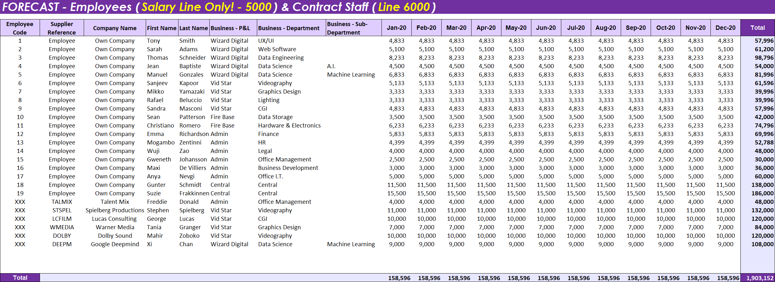
Click to view large-sized image
Note: You could go further with the forecasting here and create separate forecast tables, at a unit level, for other payroll lines such as Employer’s Tax, and Pension, and so on – as it is for the Actuals data. There is a time / effort trade-off here, depending on how accurate you want to be for each different nominal ledger line. In this case, we simplify, by forecasting for these lines later, using simple percentages on the salary line: 5000, but only after the salary line has been aggregated
Budgeted Data
We also assume that Budgeted Data (set at the beginning of the year only) is available in a similar format.
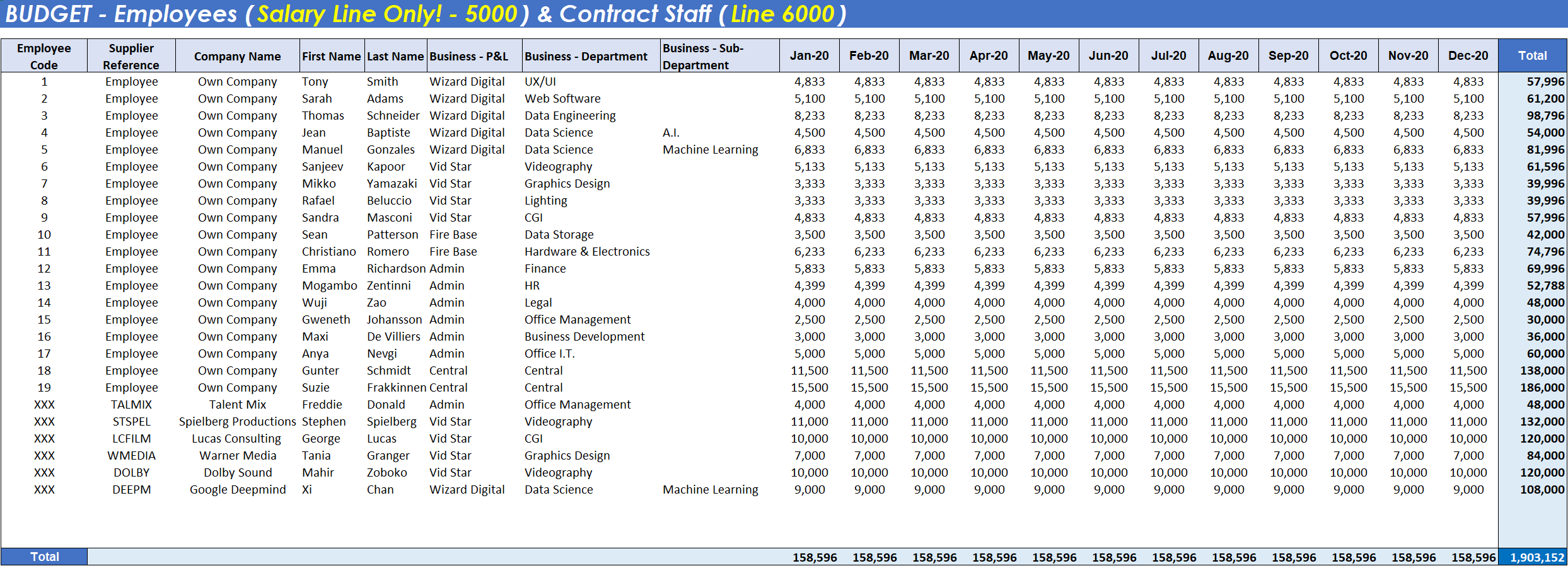
Click to view large-sized image
Note: You could go further here and create separate budget tables, at a unit level, for other payroll lines such as Employer’s Tax, and Pension – as it is for the Actuals data. There is a time / effort trade-off here, depending on how accurate you want to be for each nominal ledger line. In this case, we simplify, by setting the budget for these lines later, using simple percentages on the salary line: 5000, but only after the salary line has been aggregated
To make quick and meaningful comparisons across these 3 datasets, at both a P&L level, and Unit (Person) level, we first need to get the data into the right format. Doing this will greatly simplify any formula constructions later on – so it is definitely worth doing now! The rest of this article explains how to do this, before illustrating different methods for making comparisons and calculating variances between the datasets.
Steps
1. Transform the Actuals data
- Starting with the more detailed Actuals data, load this data into the ETL editor, so it looks like this (not all columns are shown below):
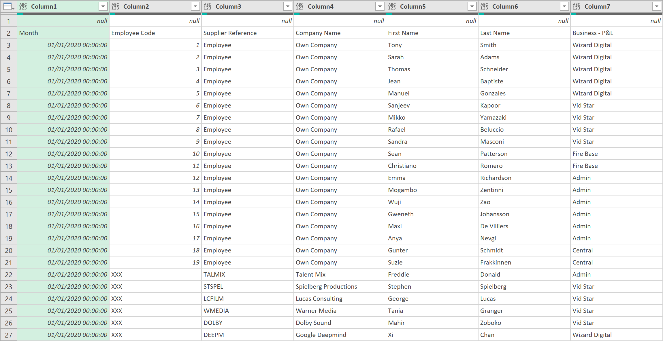
- Remove any Empty rows in the dataset with the following ‘M’-code:
= Table.SelectRows(Source, each not List.IsEmpty(List.RemoveMatchingItems(Record.FieldValues(_), {"", null})))
- Transpose the data so it now looks like this:
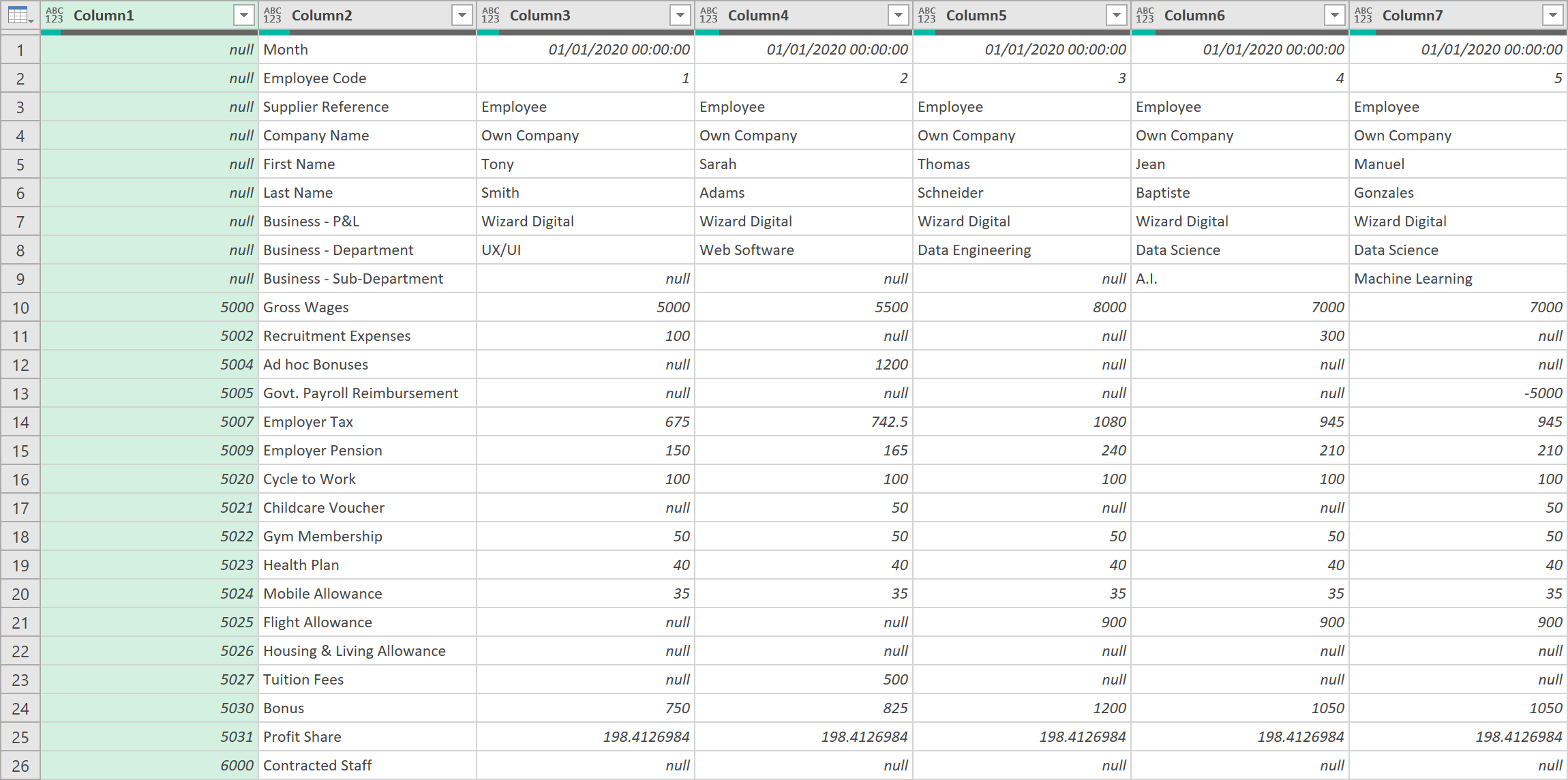
- Filter out any null rows, on Column 2
- Now, merge Column 1, with Column 2, with the following delimiter ‘=>’, so it looks like this:
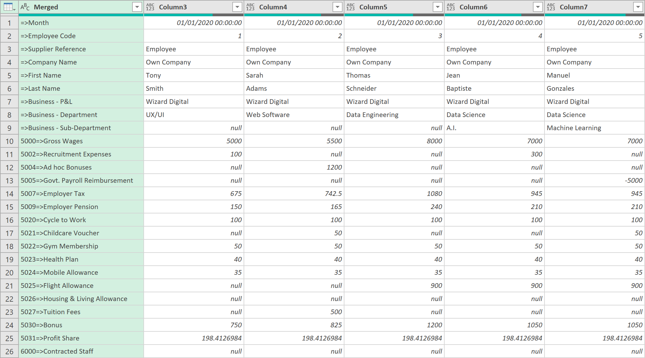
- Transpose the data back to its original format
- Next, promote the first row as headers, so the data now looks like this
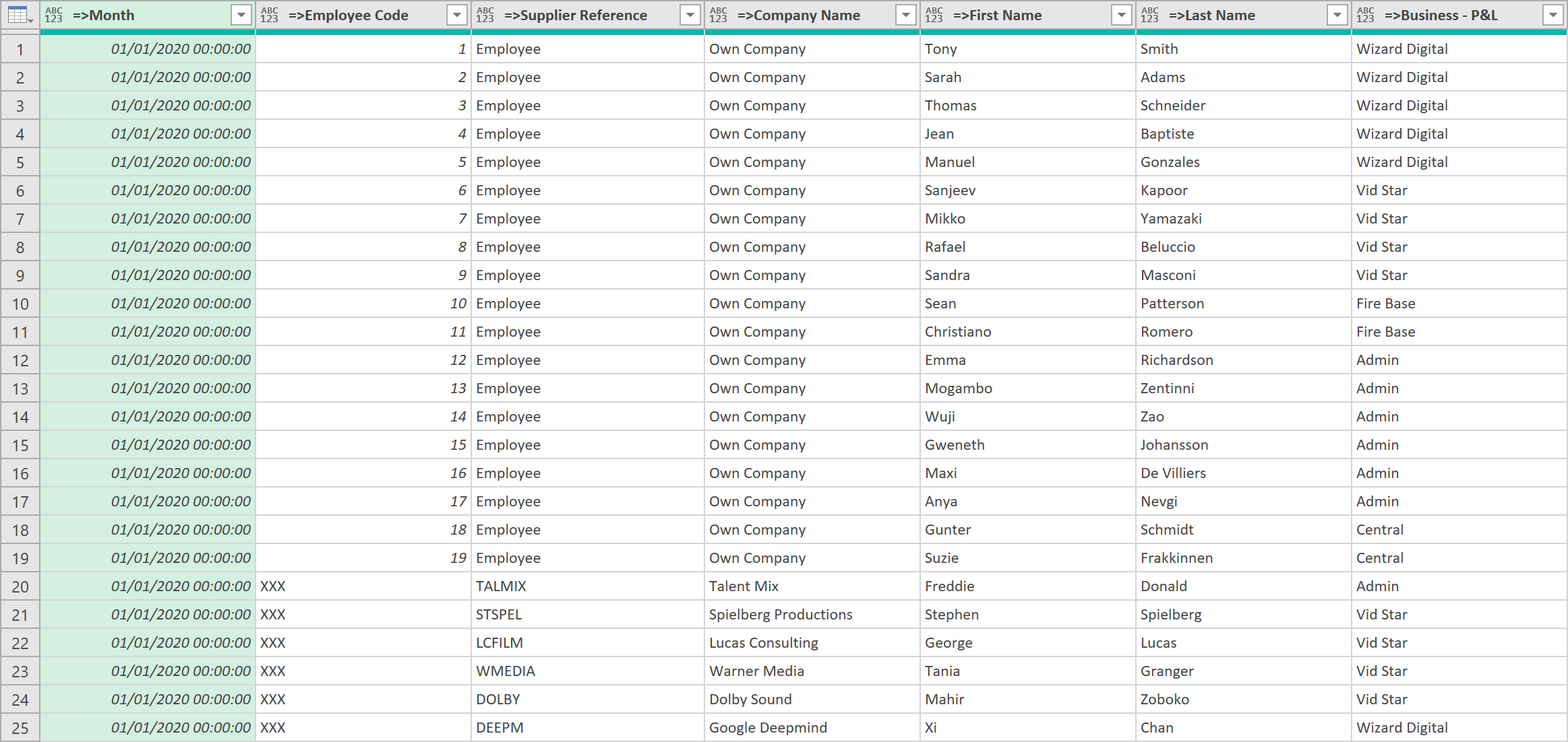
- Select all the columns that are NOT the nominal ledger columns. When selected, choose to ‘Unpivot Other Columns’
After the unpivoting step, the data should now look like this (not all columns shown), with all the values shown in one column:
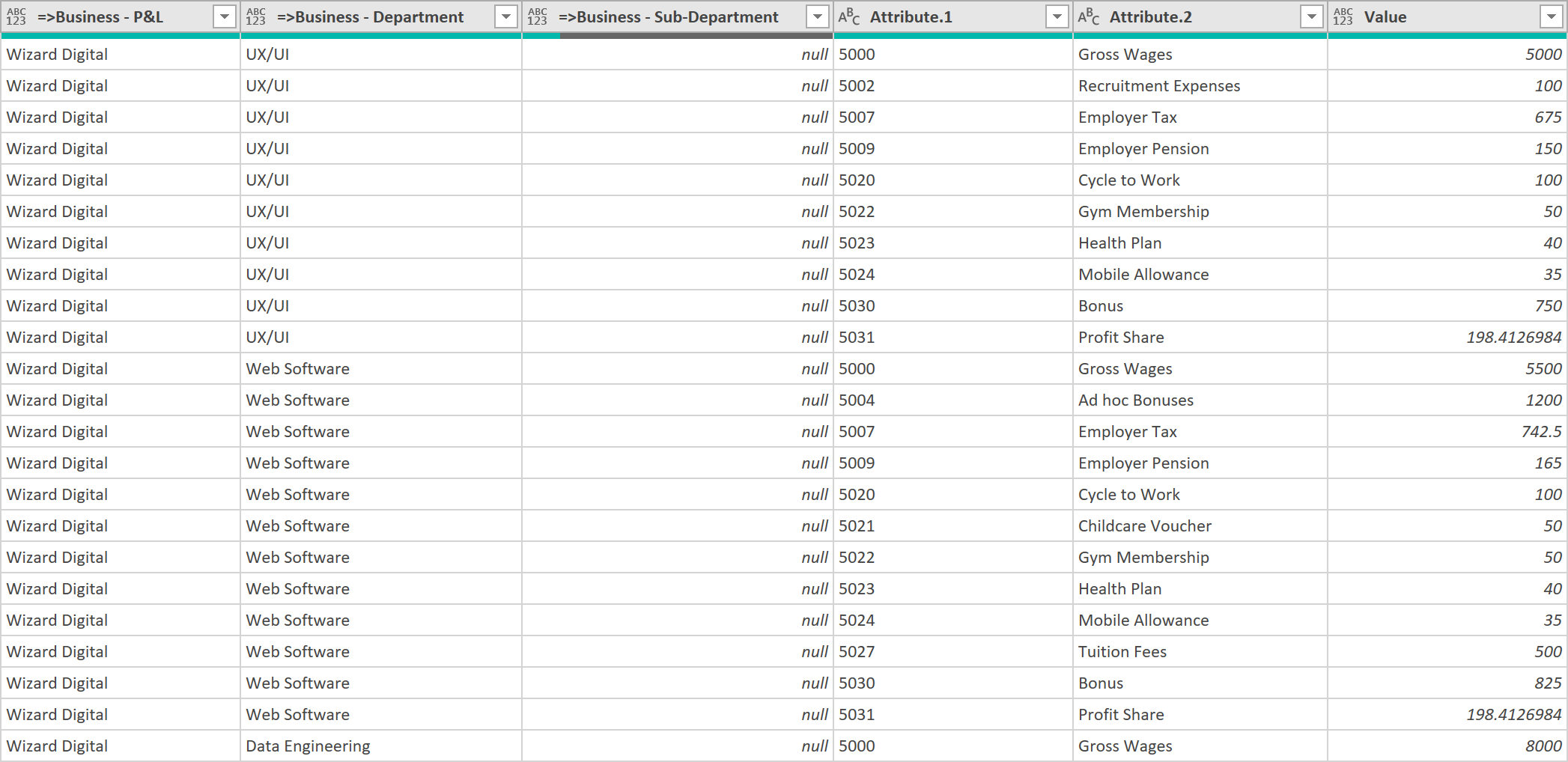
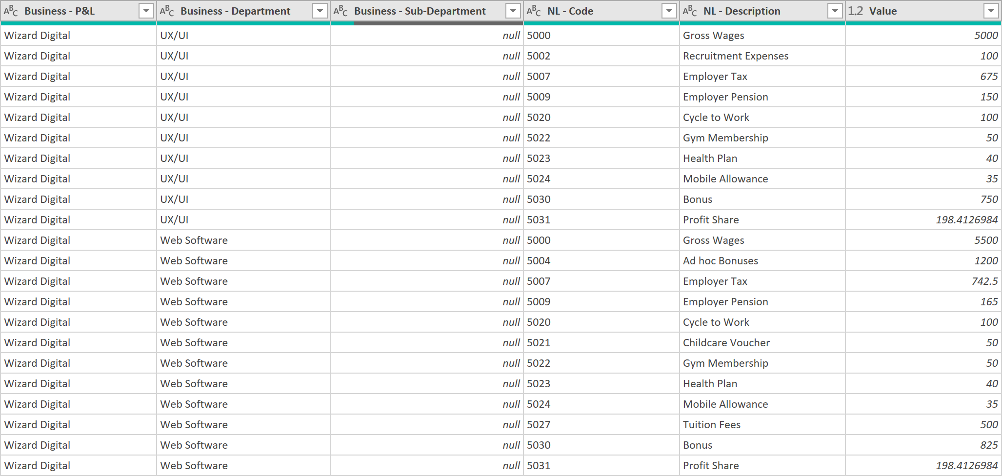
- Now, rename the column headings so you remove the ‘=>’ in the titles
- Finally, apply ‘Data Types’ to all the columns, so it looks like this:
-
Call the query ‘Jan Payroll’
-
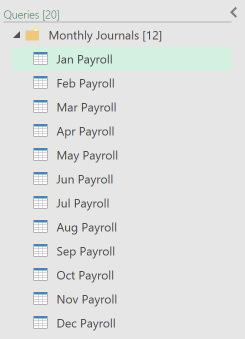
Now, repeat this process (Duplicate the query, and change the source reference in the first step) for the Months, Feb through to Dec, like shown below - (we assume you already have empty ‘placeholder’ tabs created for this, in your Excel workbook):
- After doing this, create another query that consolidates the 12 monthly queries
- Call the query ‘Actuals – Payroll (All Lines)’
- The first step of the query should look something like this, that consolidates all the monthly data:
= Table.Combine({#"Jan Payroll", #"Feb Payroll", #"Mar Payroll", #"Apr Payroll", #"May Payroll", #"Jun Payroll", #"Jul Payroll", #"Aug Payroll", #"Sep Payroll", #"Oct Payroll", #"Nov Payroll", #"Dec Payroll"})
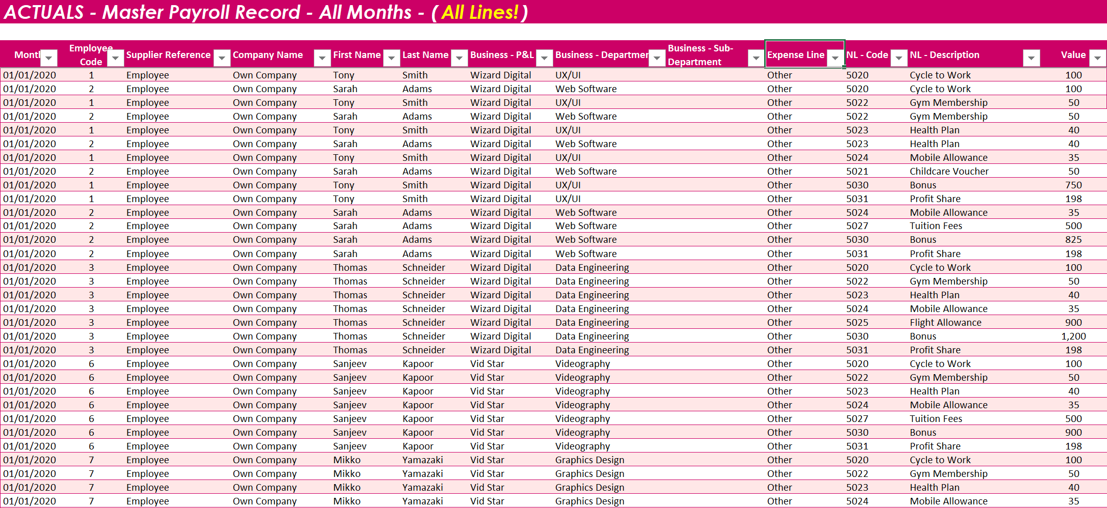
- Load the query to the worksheet, so it looks something like this:
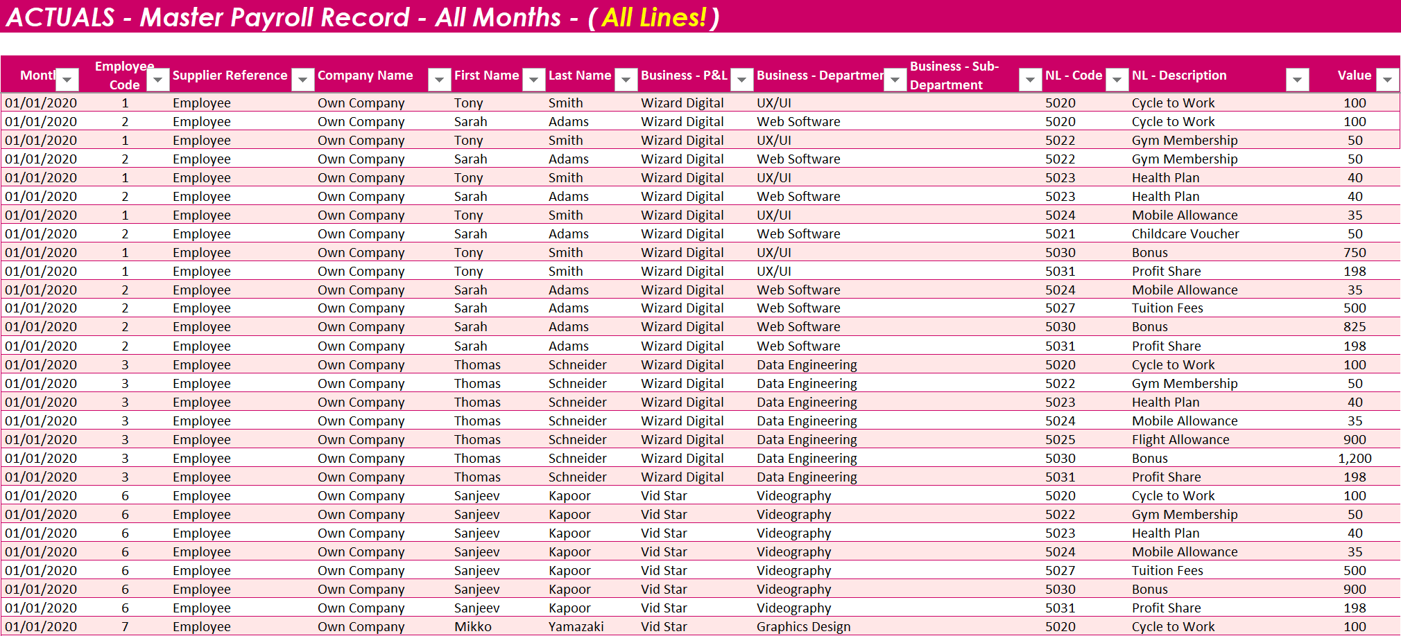
- We are almost finished with this query, we just need to add one extra column, that we define for analysis / comparison purposes ourselves, but leave this for now.
2. Create a Nominal Ledger Mapping Table
- Next, create a Blank Query called: ‘NL – Line’ – using the following code as the first step:
= Table.Combine({#"Jan Payroll", #"Feb Payroll", #"Mar Payroll", #"Apr Payroll", #"May Payroll", #"Jun Payroll", #"Jul Payroll", #"Aug Payroll", #"Sep Payroll", #"Oct Payroll", #"Nov Payroll", #"Dec Payroll"})
- Remove all columns except ‘NL – Code’ and ‘NL – Description’
- Now, remove any duplicates
- Sort the data in ascending order of ‘NL – Code’, so it looks like this:
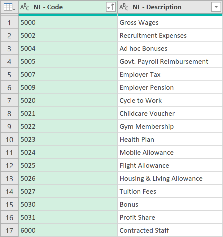
- Load this table to Excel
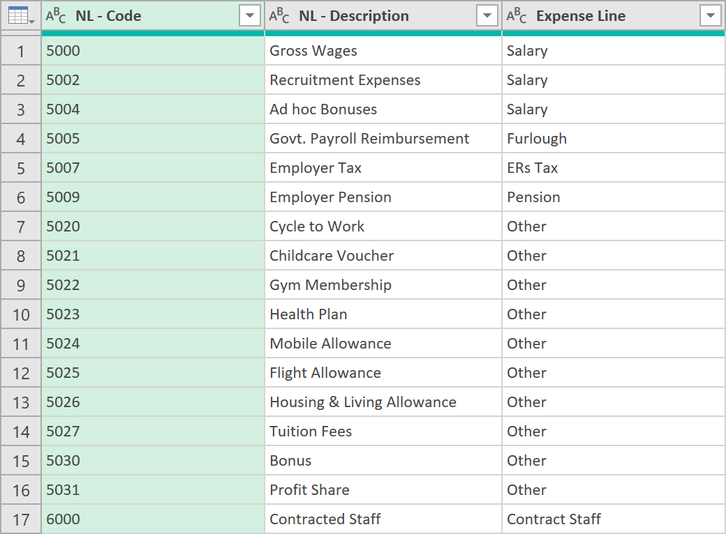
- In Excel, manually add another column to the table, called ‘Expense Line’ – and define a less granular mapping of Nominal Ledger Lines (that we will use later for analysis / comparison purposes later) like so:
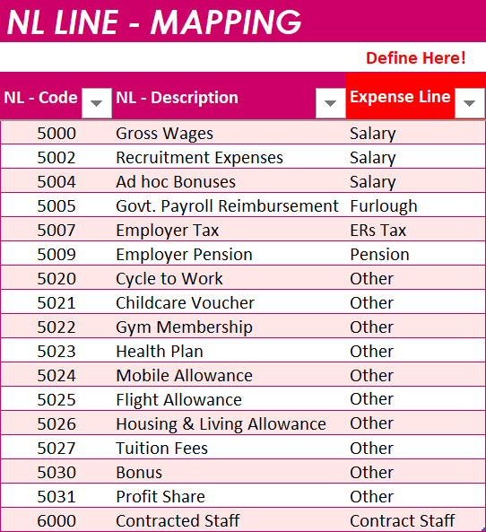
- Next, import this table (with the extra ‘Expense Line’ column) back into the ETL editor
- Call the re-imported table, ‘NL – Lines with Mapping’. After defining data types, it should look like this:
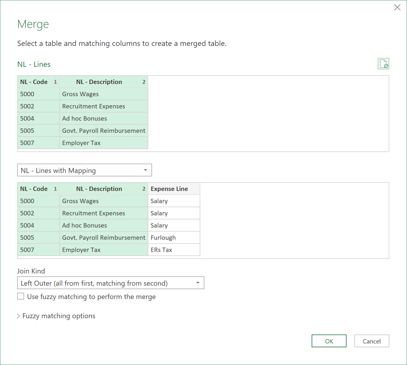
- Now, go back to the query called ‘NL – Line’ created earlier, and add a Merge Step. This step creates a logically linked, self-referencing table, so we can import the NL mappings defined earlier.
- Now, expand the ‘Expense Line’ field, so the query looks like this:
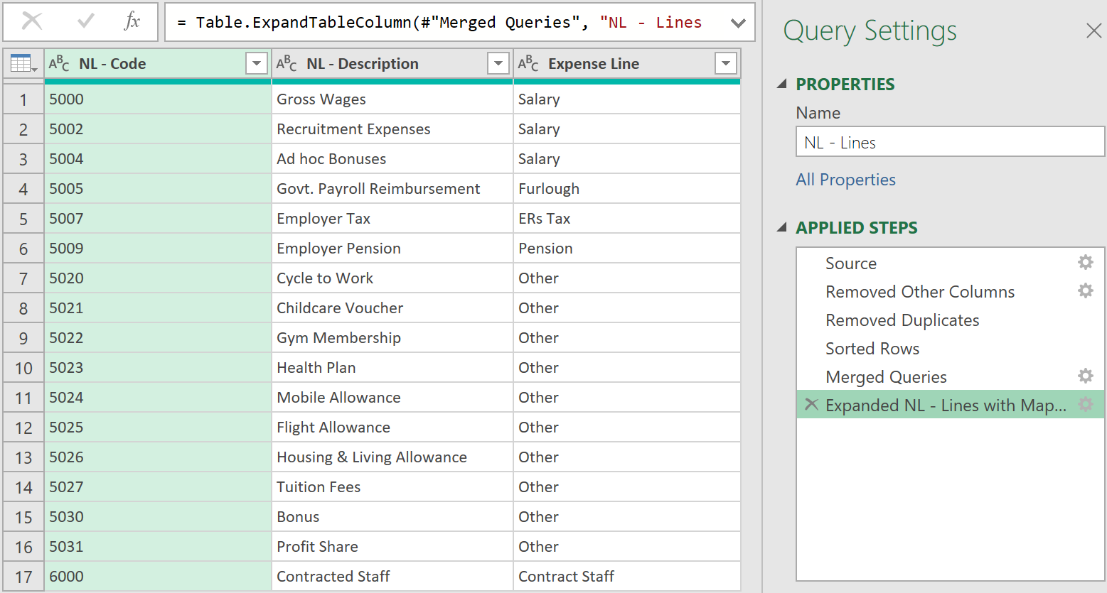
- Load the table back to Excel. (You might see a second column called ‘Expense Line 2’ automatically created – if you do, just delete it)
- The final ‘M’-code to this query should look like this:
let
    Source = Table.Combine({#"Jan Payroll", #"Feb Payroll", #"Mar Payroll", #"Apr Payroll", #"May Payroll", #"Jun Payroll", #"Jul Payroll", #"Aug Payroll", #"Sep Payroll", #"Oct Payroll", #"Nov Payroll", #"Dec Payroll"})
,
    #"Removed Other Columns" = Table.SelectColumns(Source,{"NL - Code", "NL - Description"}),
    #"Removed Duplicates" = Table.Distinct(#"Removed Other Columns"),
    #"Sorted Rows" = Table.Sort(#"Removed Duplicates",{{"NL - Code", Order.Ascending}}),
    #"Merged Queries" = Table.NestedJoin(#"Sorted Rows", {"NL - Code", "NL - Description"}, #"NL - Lines with Mapping", {"NL - Code", "NL - Description"}, "NL - Lines with Mapping", JoinKind.LeftOuter),
    #"Expanded NL - Lines with Mapping" = Table.ExpandTableColumn(#"Merged Queries", "NL - Lines with Mapping", {"Expense Line"}, {"Expense Line"})
in
    #"Expanded NL - Lines with Mapping"
3. Add the Mapped NL column to the Consolidated Actuals Query
- Now, go back to the ‘Actuals – Payroll (All Lines)’ query created earlier, and add the following Merge operation, to add the one extra column that we needed to:
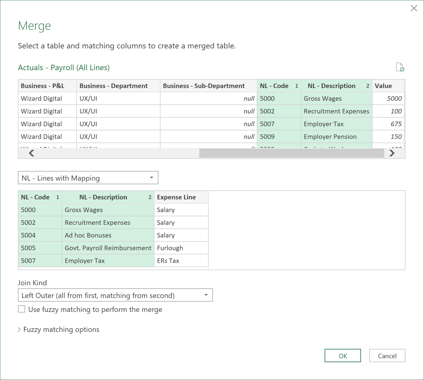
- Expand the ‘Expense Line’ field, and re-order the ‘Expense Line’ column to a more suitable place, like shown below:
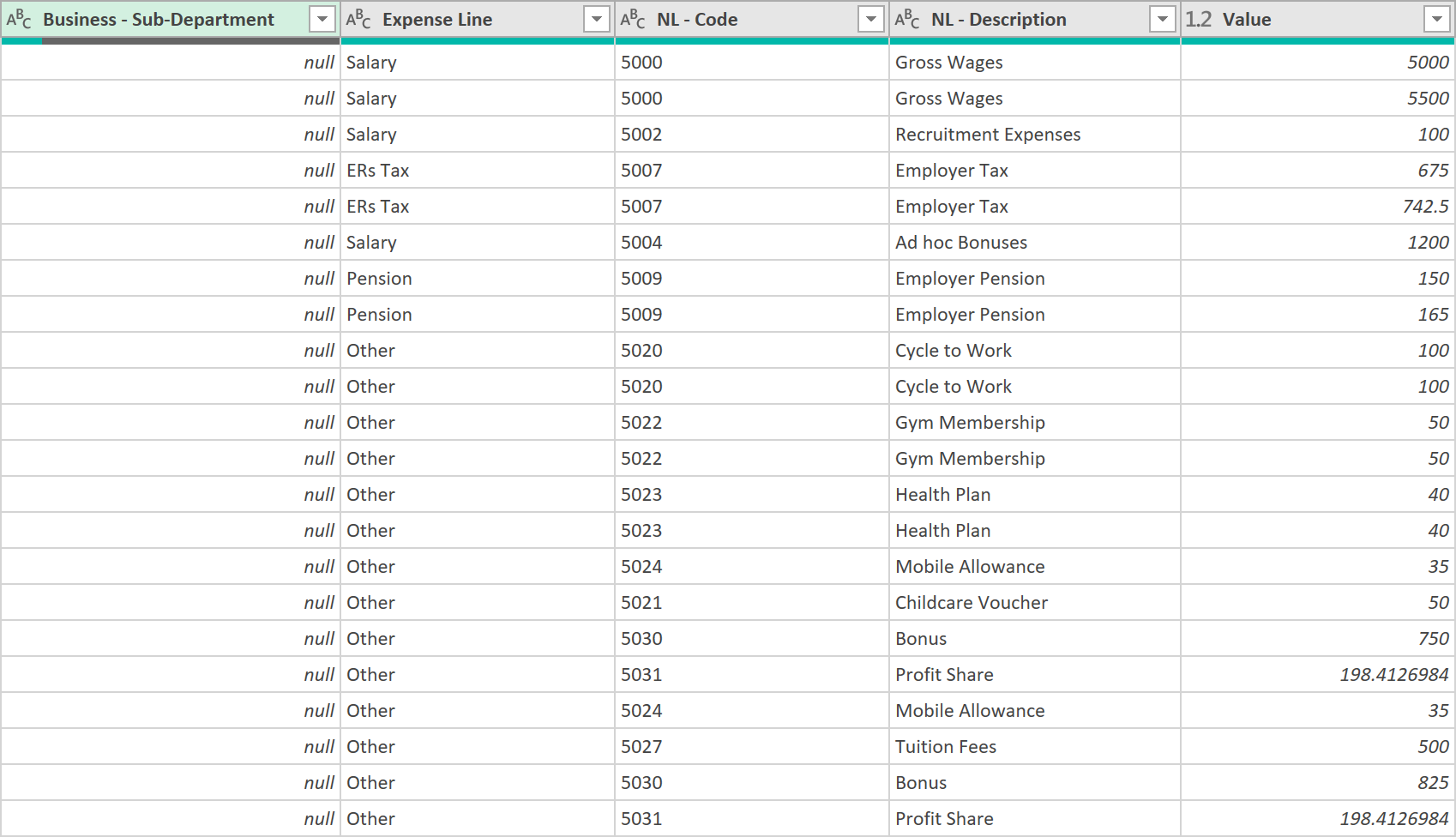
- When you re-load this query to Excel, it should now the same data as before, but with the extra column, ‘Expense Line’ – that we defined earlier, elsewhere!
let
    #"Consolidated Query" = Table.Combine({#"Jan Payroll", #"Feb Payroll", #"Mar Payroll", #"Apr Payroll", #"May Payroll", #"Jun Payroll", #"Jul Payroll", #"Aug Payroll", #"Sep Payroll", #"Oct Payroll", #"Nov Payroll", #"Dec Payroll"}),
    #"Merged Queries" = Table.NestedJoin(#"Consolidated Query", {"NL - Code", "NL - Description"}, #"NL - Lines with Mapping", {"NL - Code", "NL - Description"}, "NL - Lines with Mapping", JoinKind.LeftOuter),
    #"Expanded NL - Lines with Mapping" = Table.ExpandTableColumn(#"Merged Queries", "NL - Lines with Mapping", {"Expense Line"}, {"Expense Line"}),
    #"Reordered Columns" = Table.ReorderColumns(#"Expanded NL - Lines with Mapping",{"Month", "Employee Code", "Supplier Reference", "Company Name", "First Name", "Last Name", "Business - P&L", "Business - Department", "Business - Sub-Department", "Expense Line", "NL - Code", "NL - Description", "Value"})
in
    #"Reordered Columns"
4. Transform the Forecast data
- Now to the Forecast data. Load this data into the ETL editor, so it looks like this:
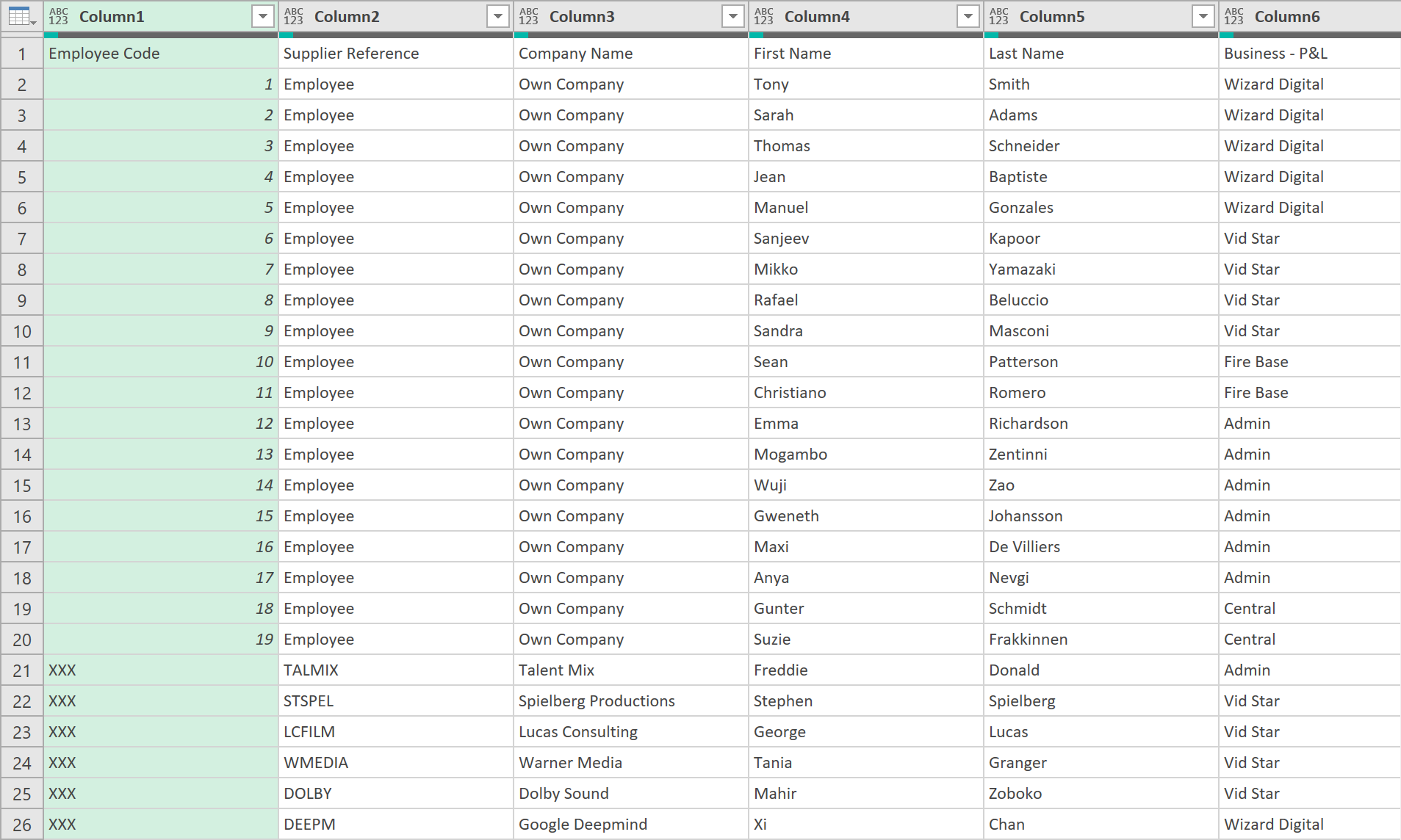
- Filter out from Column 1, any rows that have null, or the word ‘Total’
- Then, promote the top row as Headers
- Remove the Column with the title ‘Total’
- Select all columns that do NOT have dates in the column heading. Once selected, choose to ‘Unpivot Other Columns’.
- After unpivoting the data, apply the correct Data Types to each column
- Call the query: ‘Forecasts – Payroll (Salary Line)’
- Finally, load the data back to Excel, so it looks like this:
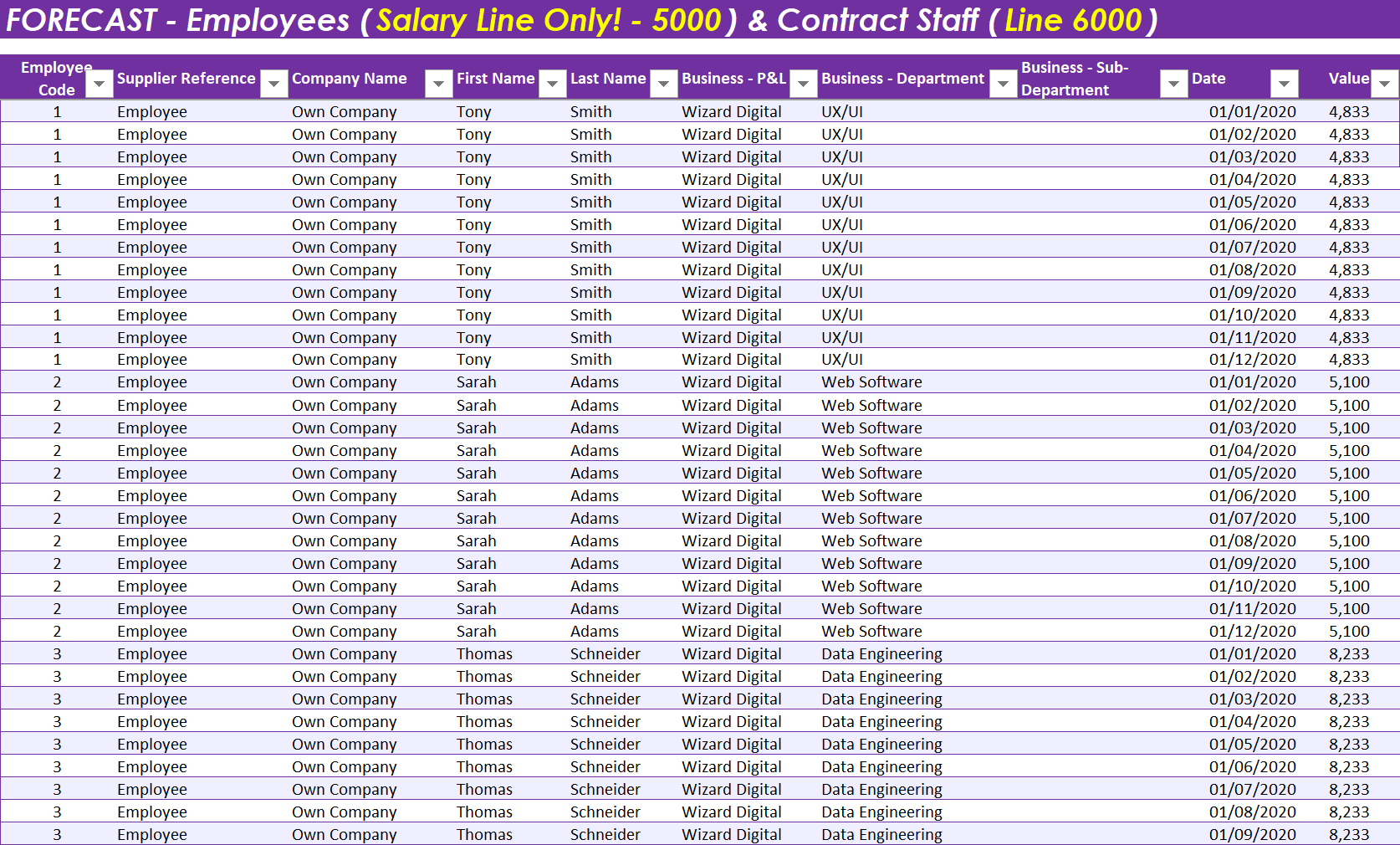
- The final ‘M’ code to the query should look like this:
let
    Source = Excel.CurrentWorkbook(){[Name="Forecast_Salary_Data"]}[Content],
    #"Filtered Rows" = Table.SelectRows(Source, each ([Column1] <> null and [Column1] <> "Total")),
    #"Promoted Headers" = Table.PromoteHeaders(#"Filtered Rows", [PromoteAllScalars=true]),
    #"Removed Columns" = Table.RemoveColumns(#"Promoted Headers",{"Total"}),
    #"Unpivoted Other Columns" = Table.UnpivotOtherColumns(#"Removed Columns", {"Employee Code", "Supplier Reference", "Company Name", "First Name", "Last Name", "Business - P&L", "Business - Department", "Business - Sub-Department"}, "Attribute", "Value"),
    #"Changed Type" = Table.TransformColumnTypes(#"Unpivoted Other Columns",{{"Attribute", type datetime}}),
    #"Renamed Columns" = Table.RenameColumns(#"Changed Type",{{"Attribute", "Date"}}),
    #"Changed Type1" = Table.TransformColumnTypes(#"Renamed Columns",{{"Date", type date}, {"Value", type number}, {"Business - Sub-Department", type text}, {"Business - Department", type text}, {"Business - P&L", type text}, {"Last Name", type text}, {"First Name", type text}, {"Company Name", type text}, {"Supplier Reference", type text}, {"Employee Code", type text}})
in
    #"Changed Type1"
5. Transform the Budget data
- As the input layout is the same, the same steps for transforming the Forecast data can be applied to the Budgeted data
- Apply the same transformations, and call the query ‘Budget – Payroll (Salary Line)’
- After loading the transformed data back to Excel, it should look something like this:
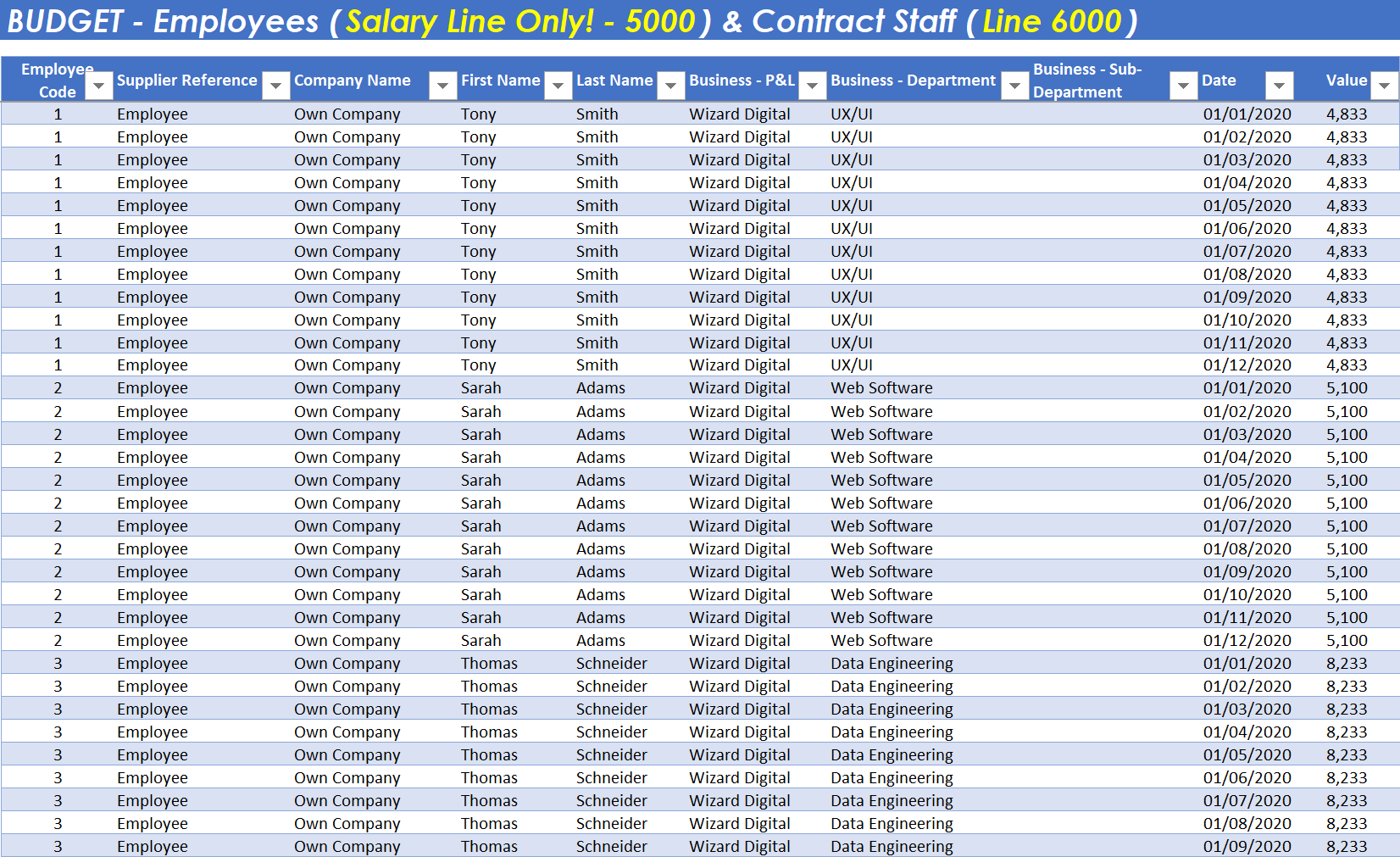
- The final ‘M’ code to the query should look like this:
let
    Source = Excel.CurrentWorkbook(){[Name="Budget_Salary_Data"]}[Content],
    #"Filtered Rows" = Table.SelectRows(Source, each ([Column1] <> null and [Column1] <> "Total")),
    #"Promoted Headers" = Table.PromoteHeaders(#"Filtered Rows", [PromoteAllScalars=true]),
    #"Removed Columns" = Table.RemoveColumns(#"Promoted Headers",{"Total"}),
    #"Unpivoted Other Columns" = Table.UnpivotOtherColumns(#"Removed Columns", {"Employee Code", "Supplier Reference", "Company Name", "First Name", "Last Name", "Business - P&L", "Business - Department", "Business - Sub-Department"}, "Attribute", "Value"),
    #"Changed Type" = Table.TransformColumnTypes(#"Unpivoted Other Columns",{{"Attribute", type datetime}}),
    #"Renamed Columns" = Table.RenameColumns(#"Changed Type",{{"Attribute", "Date"}}),
    #"Changed Type1" = Table.TransformColumnTypes(#"Renamed Columns",{{"Date", type date}, {"Value", type number}, {"Business - Sub-Department", type text}, {"Business - Department", type text}, {"Business - P&L", type text}, {"Last Name", type text}, {"First Name", type text}, {"Company Name", type text}, {"Supplier Reference", type text}, {"Employee Code", type text}})
in
    #"Changed Type1"
6. Compare Budgeted figures to Actual/Forecast figures – P&L level
Now we have the data in the right formats, it is relatively easy using standard SUMIFS formulae to compare the figures across the 3 datasets, and to then show the variances
We do this at the P&L level, as shown in the picture below:
(For the Budgeted, and Forecast data, estimates for any lines other than ‘Salary’ and ‘Contract Staff’ are done using simple percentages, rather than through an aggregation of amounts at a Unit Level)
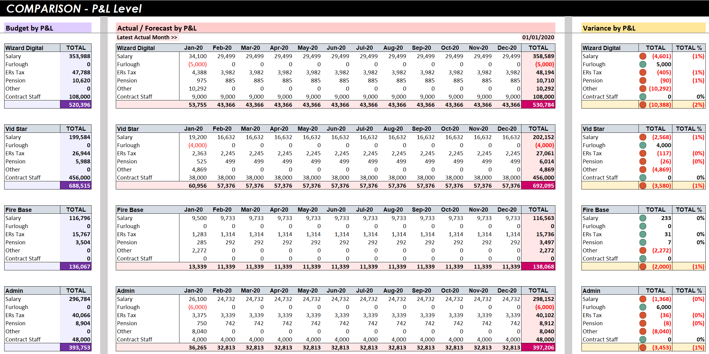
Click to view large-sized image
For the pink Actuals/Forecast table, we include a switch, so you can set the latest month for which ‘Actuals’ figures are available. Months after this date show only Forecast data, and months on or before this date show Actuals data.
The switch is built into each cell in this table, using the following formula pattern: (the specific formula below is the one applied to the ‘Salary’ line, in the Actuals/Forecast table):
=IF(
    T$7 <= $AF$5,
     SUMIFS(
          Actuals___Payroll__All_Lines[[Value]:[Value]],
          Actuals___Payroll__All_Lines[[Month]:[Month]],
          'Comparison - P&L'!T$7,
          Actuals___Payroll__All_Lines[[Supplier Reference]:[Supplier Reference]],
          "Employee",
          Actuals___Payroll__All_Lines[[Business - P&L]:[Business - P&L]],
          'Comparison - P&L'!$S$7,
          Actuals___Payroll__All_Lines[[Expense Line]:[Expense Line]],
          'Comparison - P&L'!$S8
    ),
    SUMIFS(
          Forecasts___Payroll__Salary_Line[[Value]:[Value]],
          Forecasts___Payroll__Salary_Line[[Date]:[Date]],
          'Comparison - P&L'!T$7,
          Forecasts___Payroll__Salary_Line[[Supplier Reference]:[Supplier Reference]],
          "Employee",
          Forecasts___Payroll__Salary_Line[[Business - P&L]:[Business - P&L]],
          'Comparison - P&L'!$S$7
    )
)
Finally, we’ve added a variance table to the far right so it’s easy to see the variances for each P&L, for each main line, too.
7. Download Excel File
You can download the Excel file to see how all the formulae, and switch, work, in more detail here: Payroll - Tracking - Excel File
8. Compare Budgeted figures to Actual/Forecast figures – Unit level
Comparing the datasets at a Unit (Person) level is best done through a Data Model. As new Employees or Contracts are likely to change (be added or removed) each month, it is better to make these comparisons in a dynamic way.
(You could do this statically with flat tables in an Excel sheet, but this is both error-prone, and very time-consuming to update for changes – though using OLAP Cube formulae that run off an in-built Data Model is one option you could pursue, if, for example, you needed reports with very customised layouts)
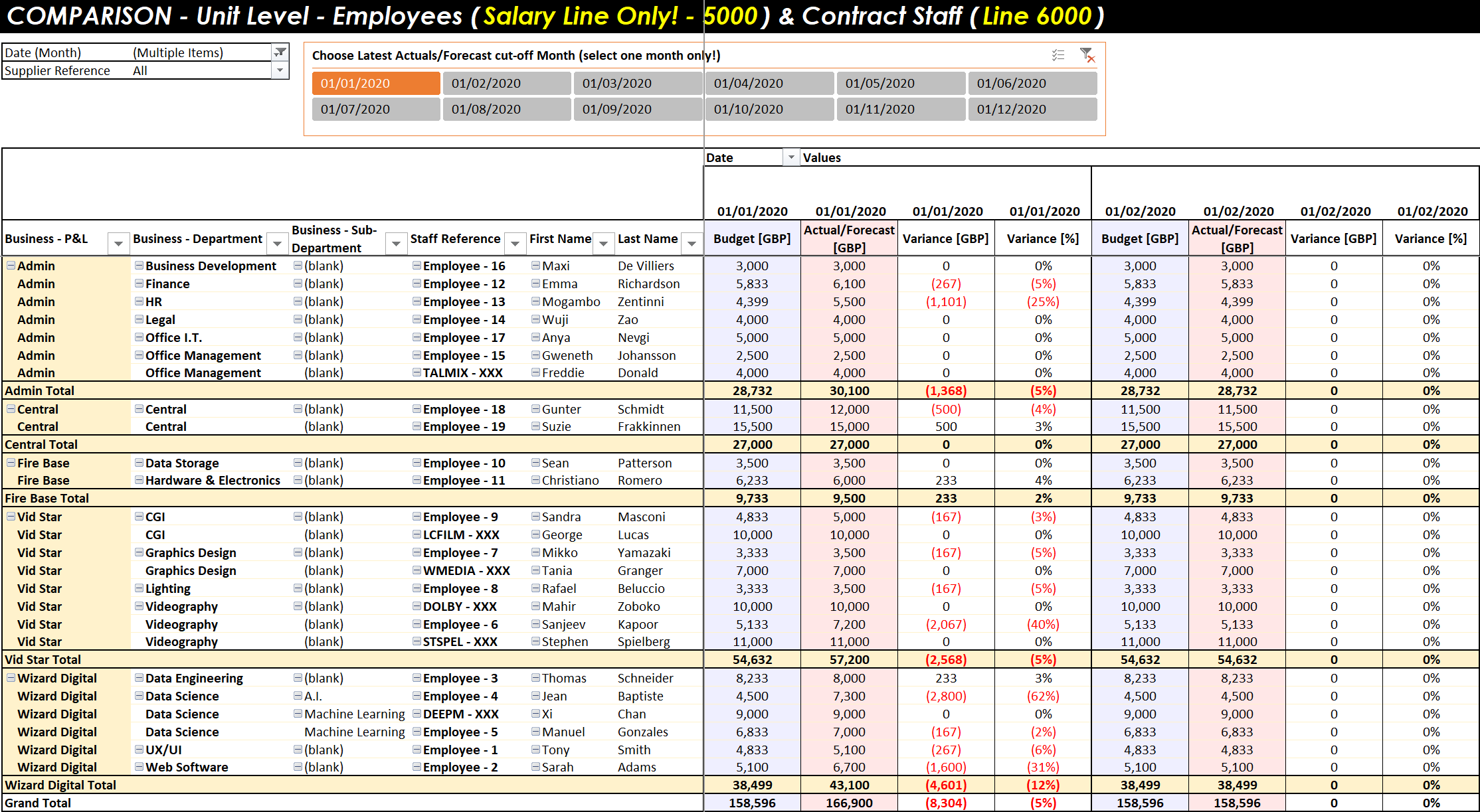
Click to view large-sized image
We show you how to do a dynamic comparison, like illustrated in the picture above, in this DAX article: Finance - Payroll Tracking.
We hope you found this article useful!
Feedback
Submit and view feedback

