Calculating tied ranks

Overview

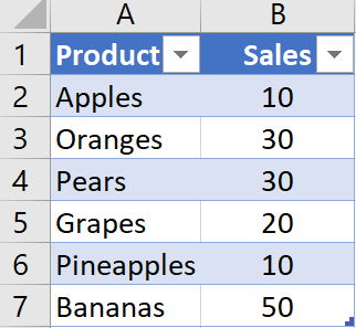
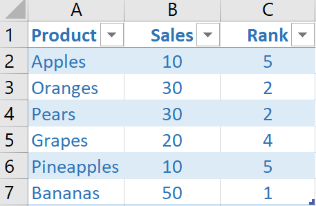
This article explains how to add a column that shows the rank of each product by its sales value. The product that has the highest sales value should have the rank 1, and products that have the same sales should have the same rank.

Steps

1. Declare a custom function

• Click inside the table in the worksheet
• Click the From Table / Range icon on the Data tab in Excel to create a new query. The Query Editor window will open and the first step in the new query will be called Source.
• Click the ƒx button next to the Formula Bar to add a new step to the query.
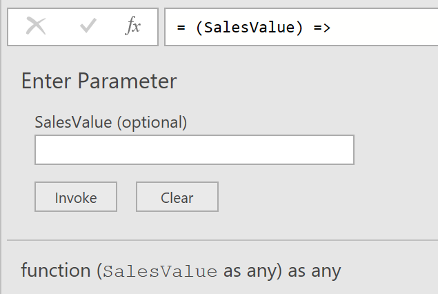
• Delete everything to the right of the equals sign and replace it with the following expression:

    (SalesValue) => Table.RowCount(Table.SelectRows(Source, each [Sales]>SalesValue) ) + 1

This expression declares a function to calculate the rank that can be called for each row on the original table. It takes a single argument, which is the sales value from the current row, and counts the number of rows in the table that have a sales value greater than the value passed in, then adds one to that number. The function can be seen below:

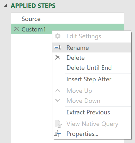
At this point the query will have two steps: one to load the data into the query, and one to declare the function. Since the name of the function is the name of the step it is declared in, rename that step to be something meaningful.

• To do this, right-click the name of the second step (at this point, called Custom1) in the Applied Steps pane
• Rename from the right-click menu, as shown below. Rename the step Rank.

2. Create a ‘Rank’ column

• Next, click the ƒx button again to add another new step to the query.
• As before, delete everything to the right of the equals sign and replace it with the name of the first step in the query, which should be called Source. This will create a new step that returns the original input table.
• Click the Custom Column icon on the Add Column tab of the Query Editor toolbar. The Custom Column dialog will appear.
• Call the new custom column Rank and enter the following expression into the Custom column formula box to call the function you have just created for each row:

    = Rank([Sales])

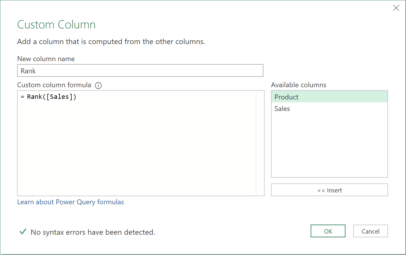
You should now see the ranks calculated correctly for each row in the table.

• Click the Close & Load button to close the Query Editor. The output of the query should be as shown below:

3. The ‘M’ code

let
    //Load data from Excel worksheet
    Source = Excel.CurrentWorkbook(){[Name="Table1"]}[Content],
    //Declare function to calculate the rank
    Rank = (SalesValue) => Table.RowCount(Table.SelectRows(Source, each [Sales]>SalesValue) ) + 1,
    //Go back to the original input table
    Custom2 = Source,
    //Add new custom column to show the rank values
    #"Added Custom" = Table.AddColumn(Custom2, "Rank", each Rank([Sales]))
in
    #"Added Custom"