Self-Referencing Tables

Overview

Here we explain how, and when it might be useful to build Self-Referencing Tables into your workbooks.

A useful practical tool: adding comments to a Debtors file

Often when you import data from a live data source, you also need to add your own commentary to that data. Sometimes you can add comments to the source file, but this is not always practical - e.g.:

• You get a new copy of the source file, each time you refresh (from your company ERP system), or because
• You are combining multiple files, and want to deal with only a cleaned, summarised view of that data (instead of all the source files directly)

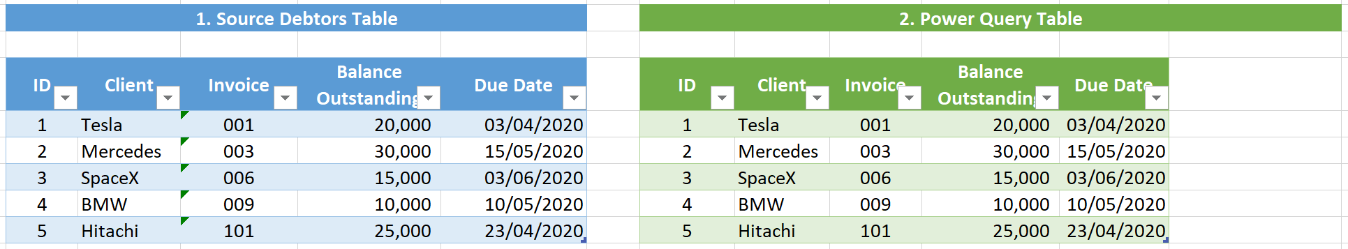
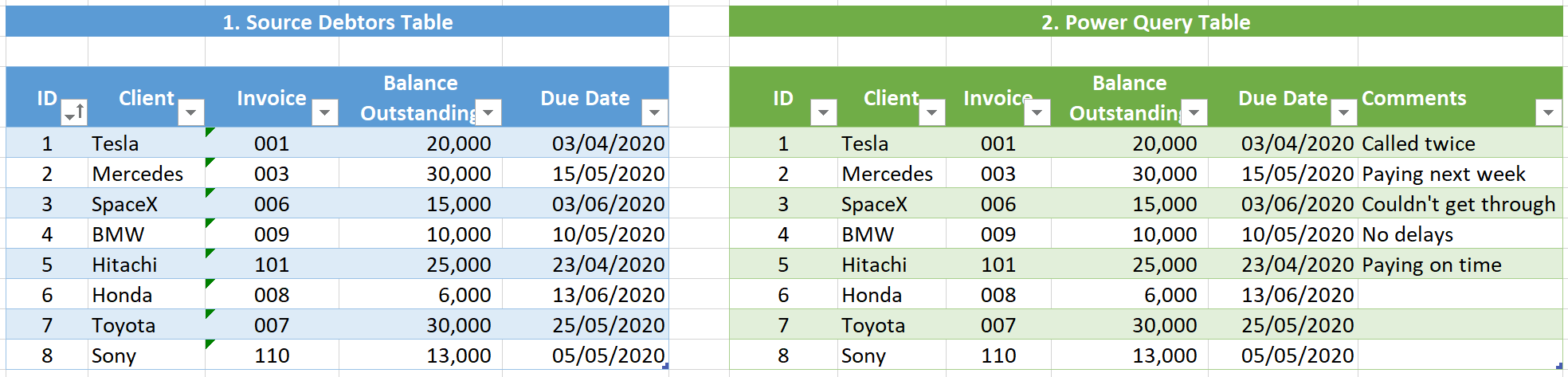
When you have loaded data from Power Query, it is possible to add a new column to the resulting loaded table (as shown below). The problem, however, is that the comments are not logically linked to the rows of data in the table.

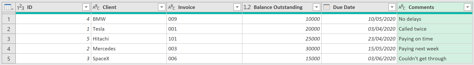
In the example below, the data is loaded from table 1 into PQ, into table 2, on the right.

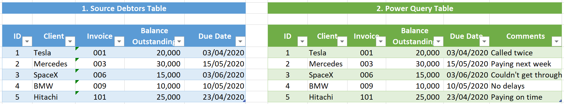
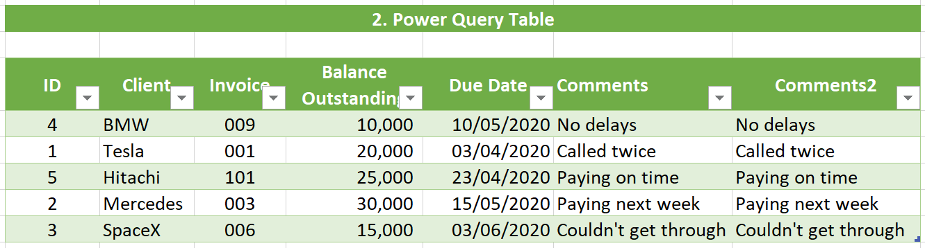
After manually adding a comments column, to table 2:

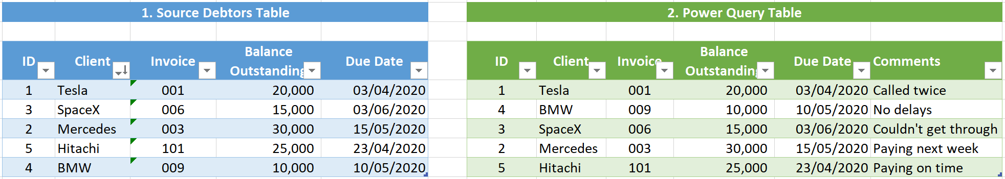
A problem however arises that if you change the order of the source table, and refresh the query, the comments will no longer align with the original data.

In the source table below, for example, the client column has been ordered alphabetically. The order of comments in the query table, after refreshing it, however, has not changed (the comment ‘called twice’ is now aligned against BMW, when it was earlier against Tesla).

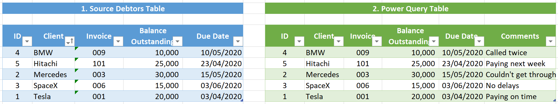
The above problem stems from the fact that the comments column added are just next to the table, rather than part of the rows of the main table.

The way to overcome this is to create a Self-Referencing Table. That is, to load table 2 above, but this time with the comments, back into the Query Editor, and then join the comments column back to the original query that was loaded. Doing this will then logically link the comments to the rows of the main table.

Steps

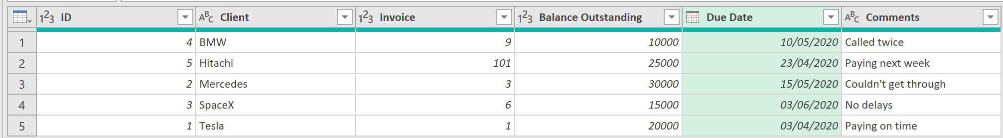
1. Load the Table with the comments back into PQ

To start, load table 2, with the comments, back into the Query Editor.

• Click any cell in the table ➔ Data tab (in Excel) ➔ From Table / Range icon

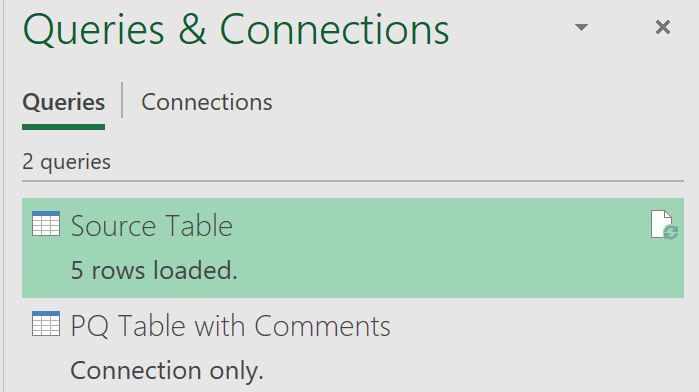
• Close and Load the table as a Connection, so you now have the following two queries in the workbook: the original query, that took data from the source table; the query that was created, called ‘PQ Table with comments’

2. Join the Comments column back to the original query

• Now, go back to editing the Query, called ‘Source Table’
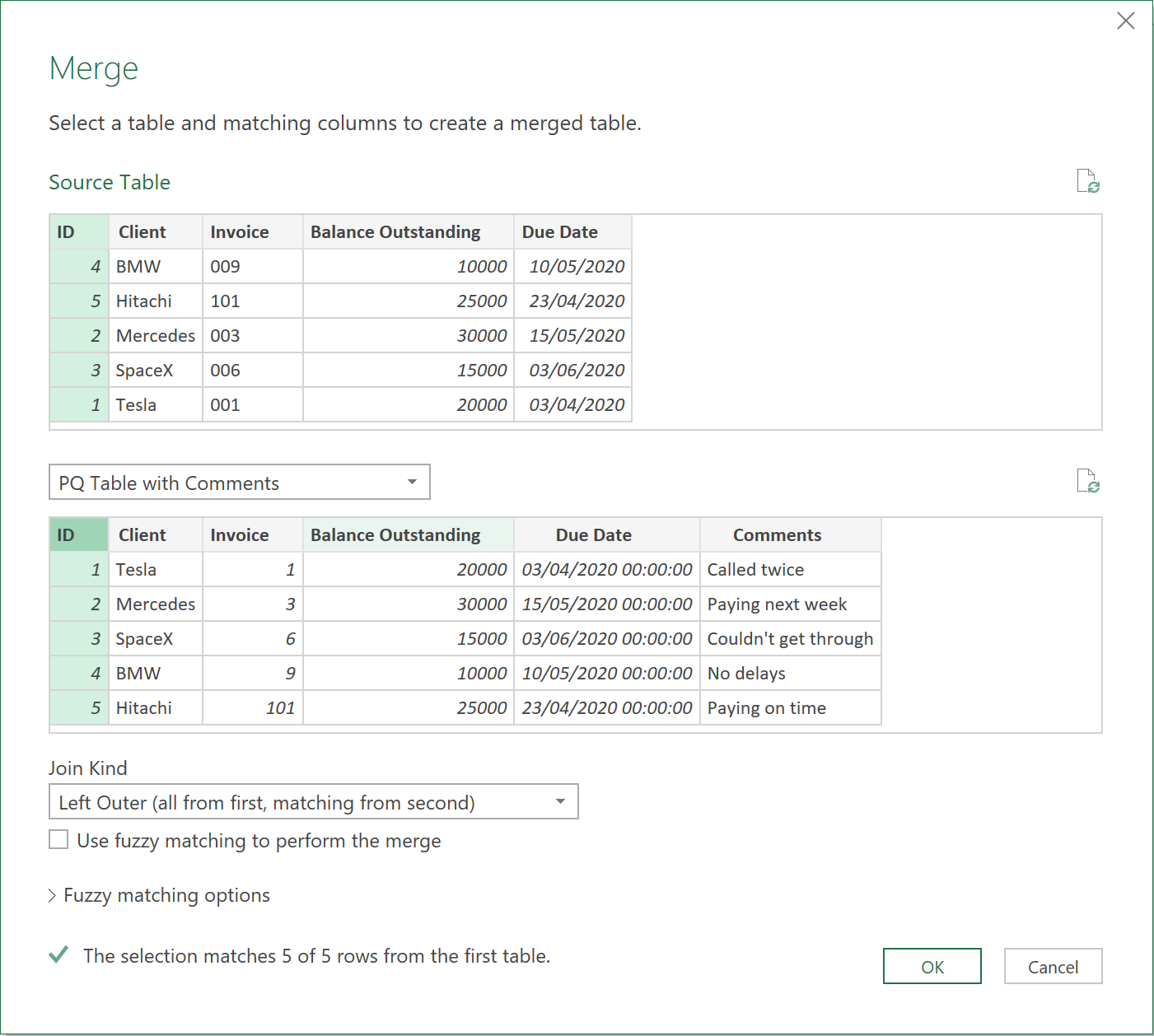
• Click Merge Queries, and choose the ‘PQ Table with Comments’ as the Query to Merge with.
• Merge on the ‘ID’ column, as shown below:

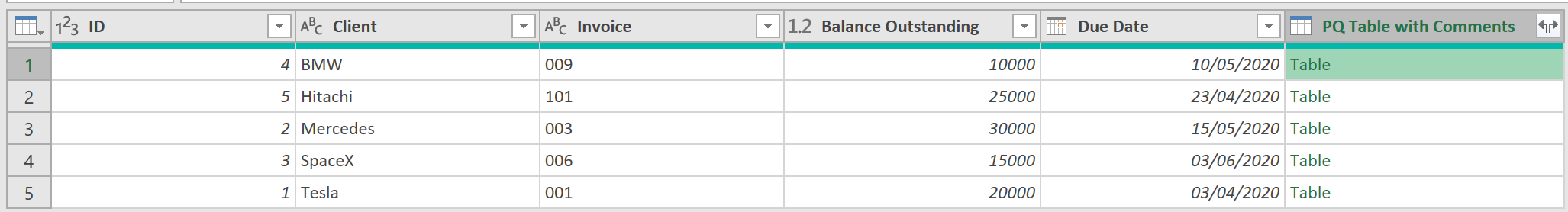
You should see a new column, with a new Table object loaded to each row

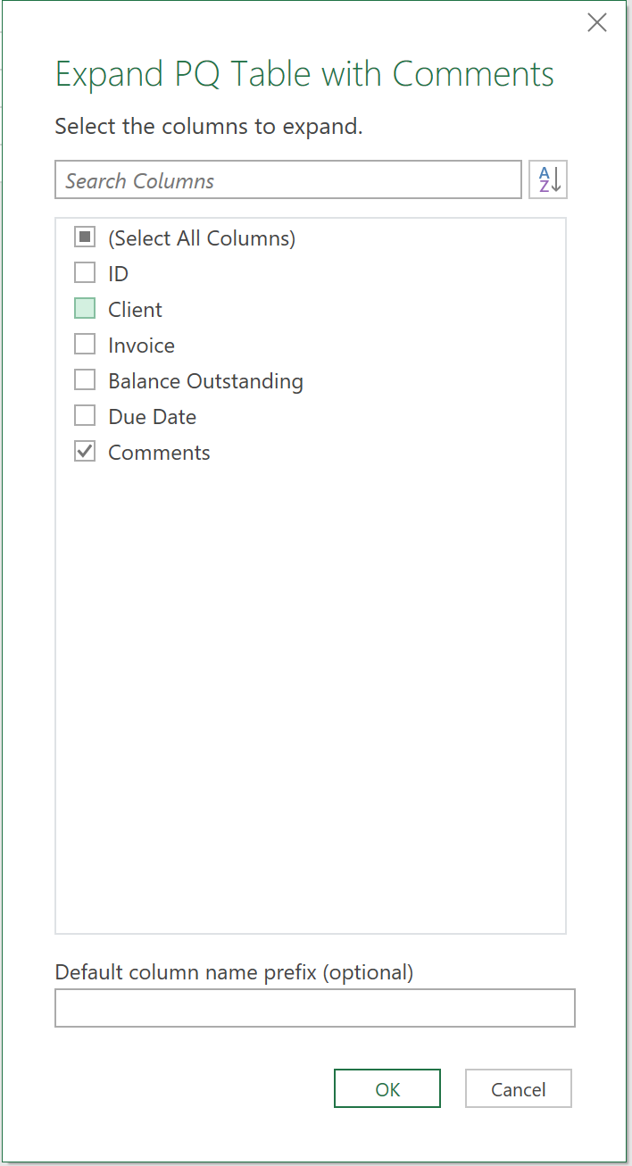
• Expand the new column, choosing to load the ‘comments’ field only, and remembering to uncheck the ‘use original column name as prefix’ option

The Query should now look as follows, with the comments loaded into the last column:

3. Delete the (duplicate) Comments column, manually added earlier

• Close and Load the query.
• Back in the Excel worksheet, you will see two comment columns. One that was just loaded through the Query, and the other that was manually added from before.

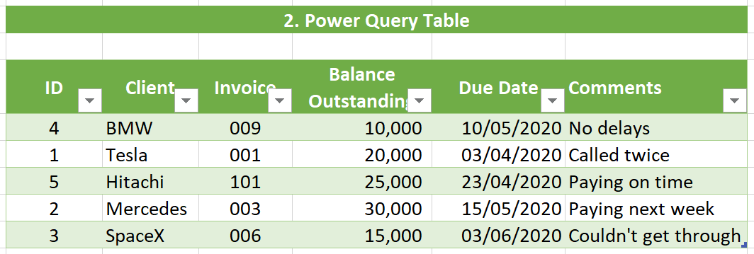
• Delete the column that was manually added before, (called ‘Comments2’ in the picture above), leaving you with a table that looks like the following. The important difference now, is that the Comments column is now logically linked to the rows of the main table, and not just added to the side of the table.

4. Test the Self-Referencing Query

Now, if you the change the order of the source table, e.g. set it to be in reverse alphabetical order, the comments in the PQ table, when you refresh it, will also align to the correct rows. The comments are logically linked through the ‘ID’ column (which holds unique values).

If you later add more items to, or change the source table, the Power Query table, with any comments that have been keyed in, will automatically align to the correct rows.

You have now successfully created and tested a Self-Referencing table!