Transition Tables

Overview

Here we explain how, and when it might be useful to use Transition Tables, in your workbook deployments

Using Transition Tables when working with Changeable Table Headers

Excel Tables are fantastic! They were a great development when Microsoft first introduced them way back in Excel 2007, as it made it much easier to organise, but importantly reference large chunks of structured data. One issue with Excel tables, however, is that they lock down the header row into hard-coded values. This in turn prohibits you from having changeable headers on your tables, that can be driven by formulae.

Consider the spreadsheet below showing the user subscriptions of a small media company. A user is able to change the year in C1 and update all headers in rows 3 of the document:

Here, we wish to load and unpivot the data (rows 3:7), but there are some challenges that need to be overcome, before this can be done.

• Putting the data in an Excel Table would cause the column headers to be locked in, and you would not be able to change the headers with any formula
• Loading the data using a Named Range would allow the column headers to change in the worksheet, but would break any hard-coded steps in the query when the date changes

To solve for the above, you need create a Transition table. This effectively puts the changeable headers of the above worksheet, into a column of a new Excel Table, and then merges this back into a query. The full process is decribed below.

Steps

1. Create a Transition Table

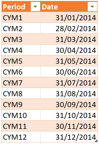
Create an Excel Table, like as follows:

To merge this into another table, you need Power Query to know that it exists. Follow these steps:

• Select any cell in the table
• Create a new query ➔ From Table/Range icon
• Select the Home tab ➔ Close and Load to… ➔ Only Create Connection

2. Retrofit the Source table

Next, to merge the data together, you need to have headers consistent with the CYM format.

• Insert a row below row 3.
• Then copy and transpose paste the values in the Period column, from the Excel Table created earlier.

Next, select rows 4:8, as you don’t want to lock row 3’s formulas. Follow these steps:

• Click inside the data range ➔ Insert ➔ Table
• Adjust the range to read ➔ =$B$4:$N$8
• OK ➔ set the table name to Customer_Data
• Hide row 4

The table should now look like this:

3. Merge the two Tables

You now need to merge the tables:

• Click inside the Customer_Data table ➔ create a new query ➔ From Table/Range
• Right click on the first column ➔ Unpivot other columns

The data is now ready to be merged.

• Go to ➔ Merge Queries icon
• Pick the Transition table
• Choose the Attribute and Period columns ➔ OK
• Expand the Date field (only) from the new column (unchecking the prefix option)
• Right click the Date column ➔ Change Type ➔ Date
• Right click the Attribute column ➔ Remove
• Right click the Value column ➔ Rename ➔ No. of Customers
• Give the first Column an appropriate name
• Change the query name to Budget
• Go to Home ➔ Close & Load

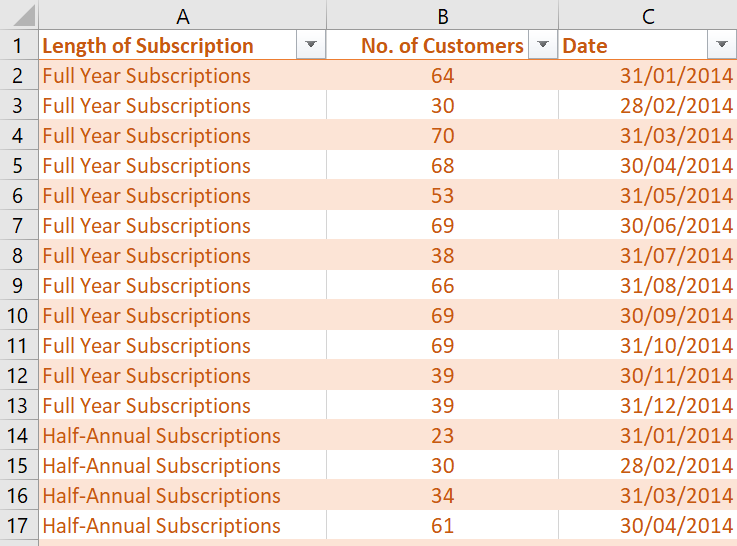
The output produces an unpivoted set of data, with the correct dates associated with each subscription type

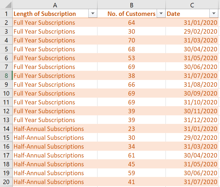
Now, if you update the year to 2020, as shown below…

…refreshing the query, should also update the years in the unpivoted dataset!