Pivoting data to enable validation

Overview

Sometimes it can be helpful to pivot into separate columns, so that, for example, separate validation dropdown lists can be created and used elsewhere in your workbook.

Consider the following data:

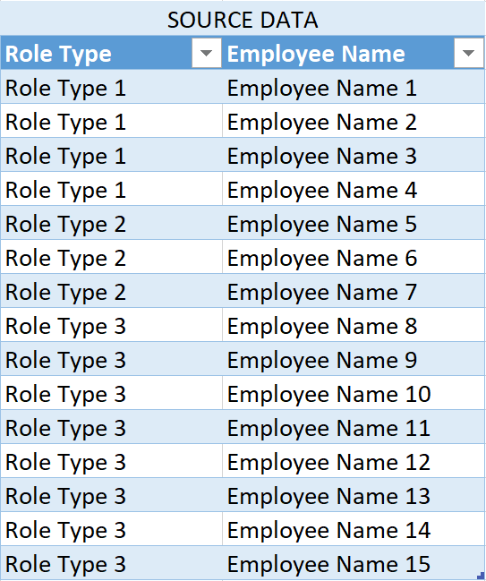
This article explains, how by using a query, such data can be reshaped, so that if you’re working with a live data source that frequently changes, you can ensure your dropdown lists stay upto date!

Steps

1. Load the data to Power Query

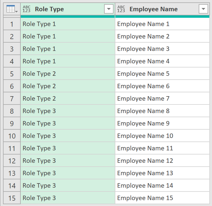
• First, load the data to power query, by clicking anywhere in the table, and then clicking on the From Table/Range icon under the Data tab in Excel

The data should load into the Query Editor as follows:

2. Group table with index row

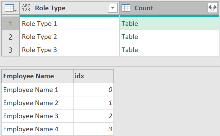
• Now, group the data by clicking on the fx icon, and entering the following code:

= Table.Group(Source, {"Role Type"}, {{"Count", (_) => Table.AddIndexColumn(_[[Employee Name]],"idx"), type table}})

This line of code will group the table, by the column ‘Role Type’. Instead of returning a count of employees in each category, it will return a table with a list of employees belonging to the category, together with a new Index column that counts up to the number of employees in each category.

• Expand all the fields in the ‘Count’ column, as shown below:

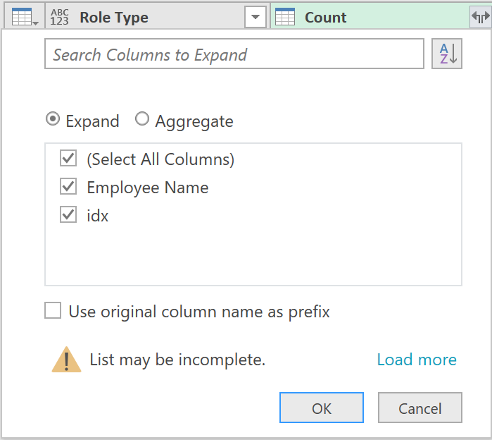
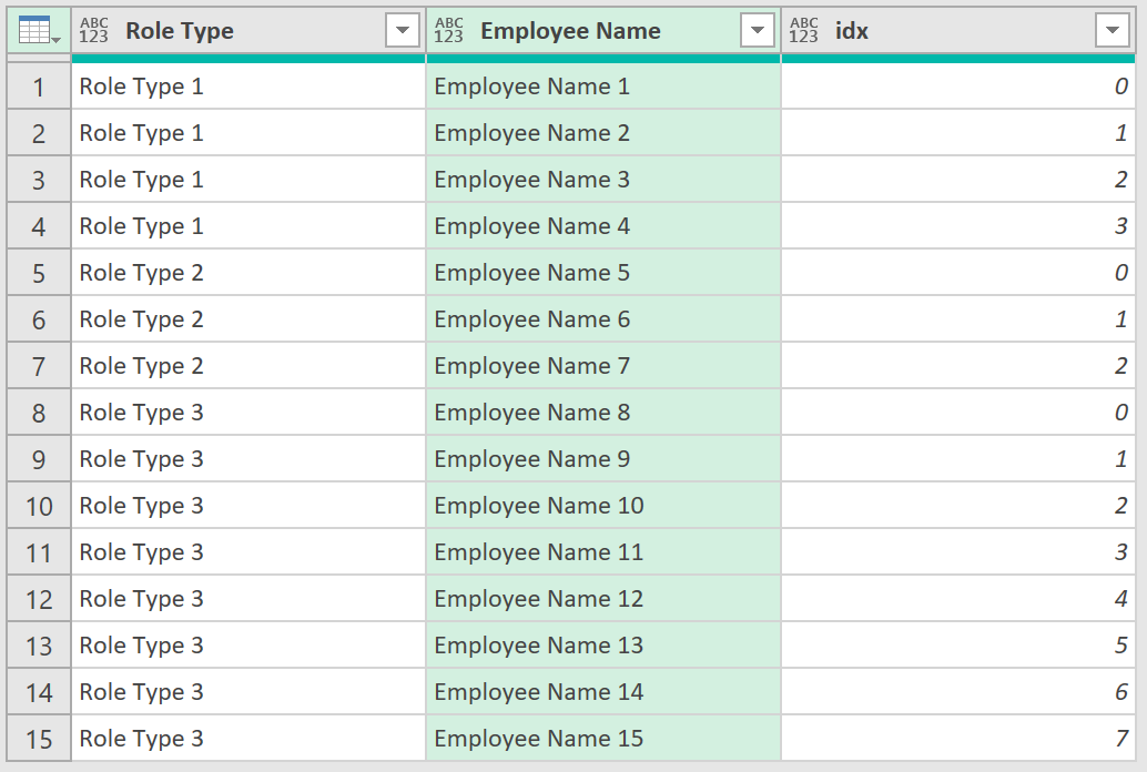
After expanding the columns, the data should now look like this:

3. Pivot the data

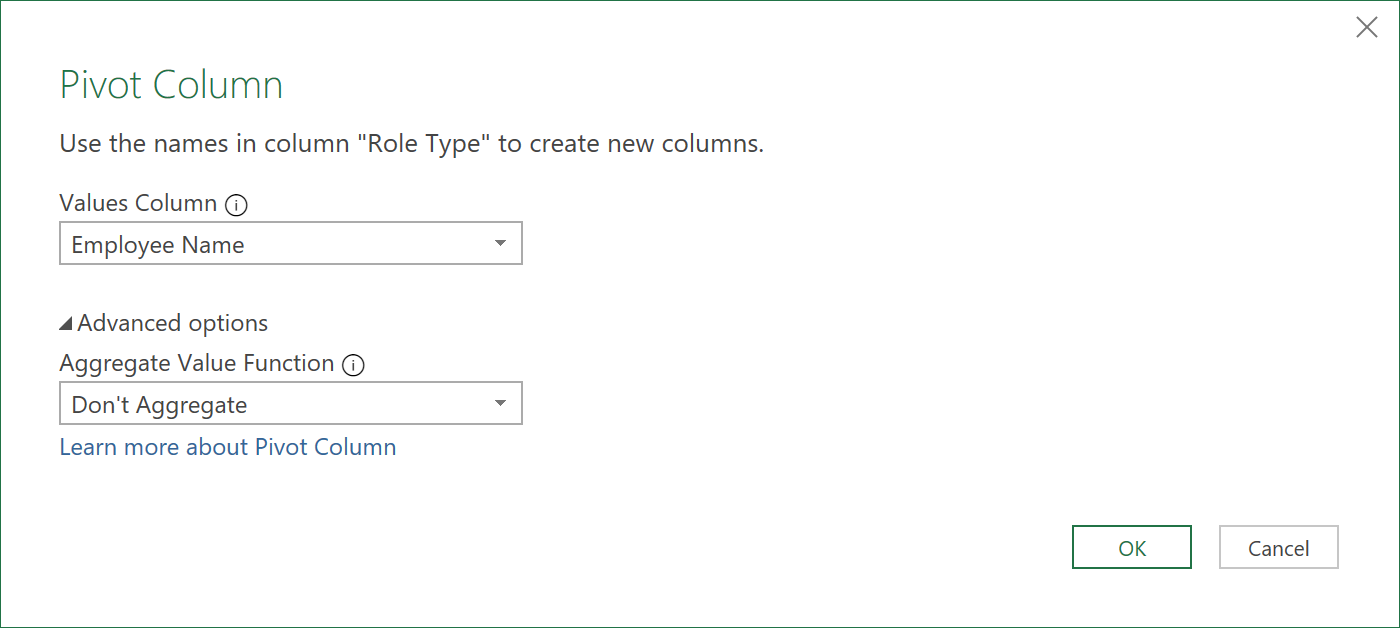
• Next, click on the ‘Role Type’ column, and then click on the ‘Pivot Column’ icon under the Transform tab
• Apply the following Pivot Column settings in the dialogue window that appears:

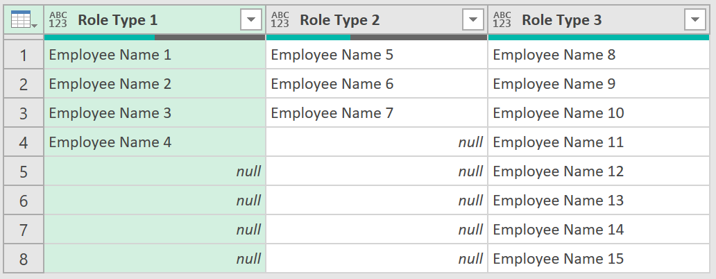
• After doing this, remove the ‘idx’ column from the pivoted data, as it is no longer needed.

The data should finally now be in a format where separate validation lists can now be created:

• Click ‘Close & Load’ to return the results to Excel