
Pivoting Text Data
Overview
Here we explain a technique for pivoting non-numeric text data.
Pivoting Text Data
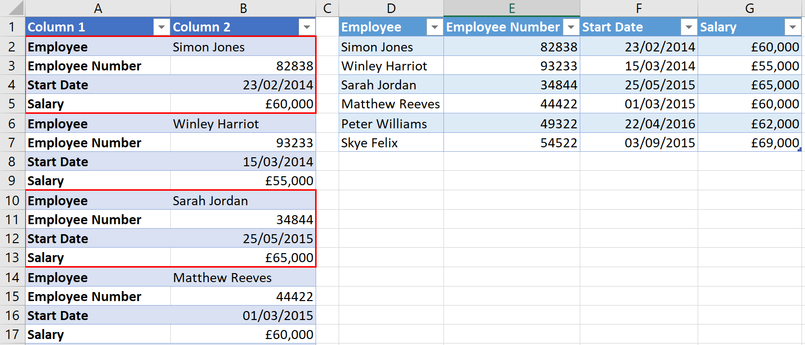
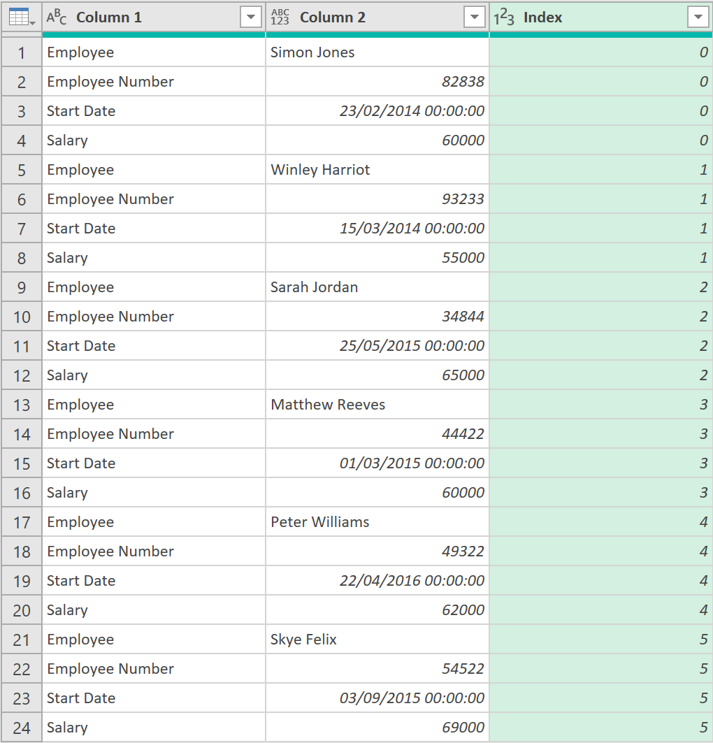
Often data needs to be transformed into a particular ‘shape’ before it can be used for further analysis, such as in the tables below, where the table on the left-hand side needs to be transformed into one that looks like the one on the right-hand side.
In the left-hand side table, column A contains the attribute, and B the values, and every 4 lines of data is a record. This kind of transformation problem is very common with older systems, when you cannot change the format of the extracted data.
You cannot pivot Text Data directly
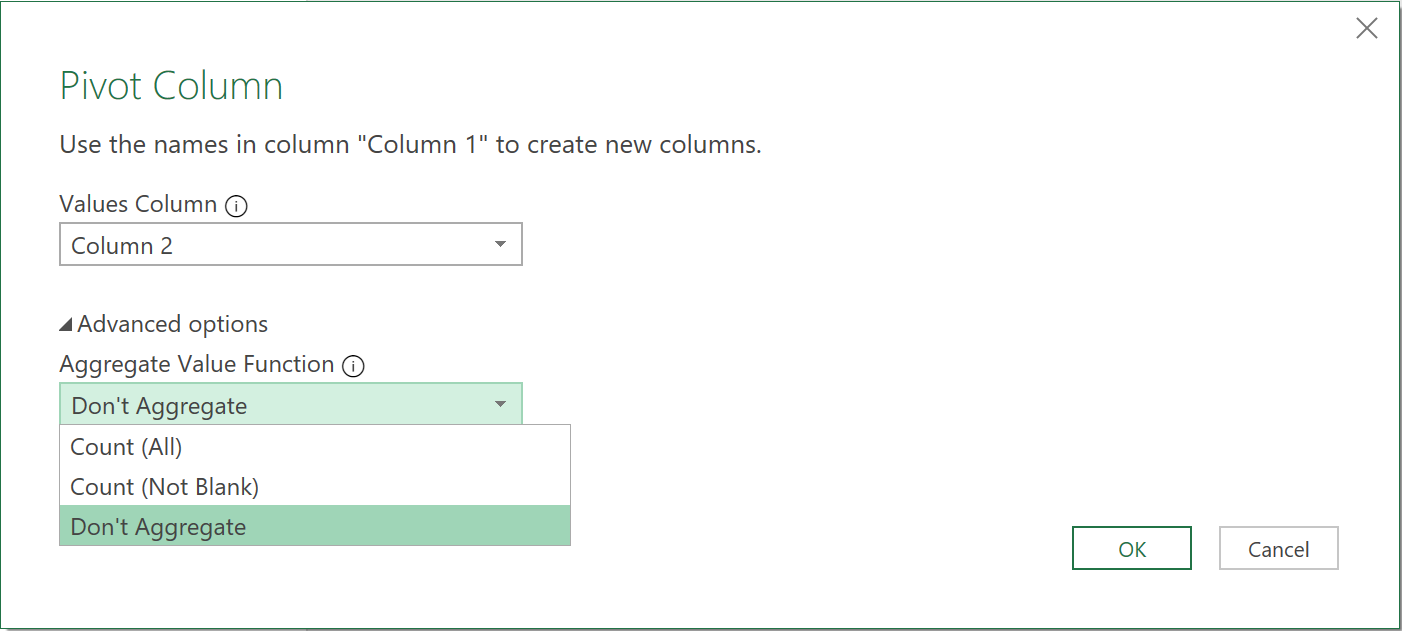
This is NOT how to do it. If you click on Column A above, in Power Query, and select ‘Pivot Column’, you will get the following results:

This approach won’t work, because Power Query does not know how to uniquely identify each record set.
Steps
In the data above, every 4 consecutive rows represents a record. So you need to assign every 4 rows with a next ID number. This unique ID number can then be used, to pivot the data on, to produce the desired results.
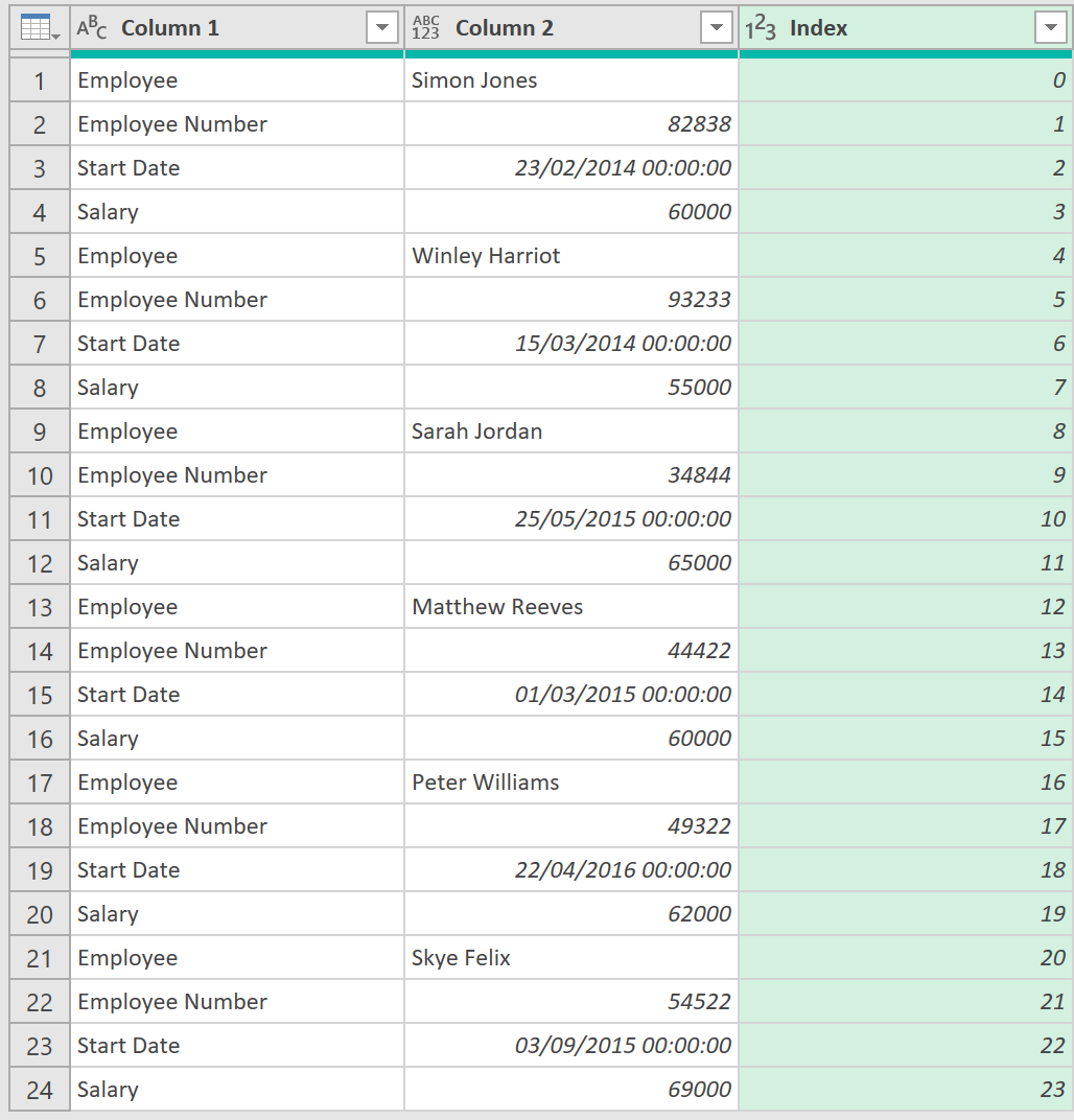
1. Add an Index Column
- Click anywhere in the Table ➔ go to the Data tab (in Excel) ➔ click the From Table / Range icon.
In the Query Editor, add a new Index Column.
- Go to the ‘Add Column’ tab ➔ click the ‘Index Column’ icon
- Choose to add the ‘Index Column’ starting from ‘0’
2. Divide the Index column by 4
- Click on the Index column ➔ go to the ‘Transform’ tab ➔ click on the ‘Standard’ icon
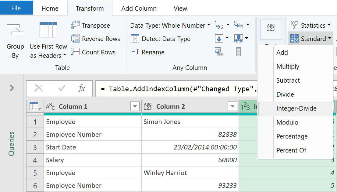
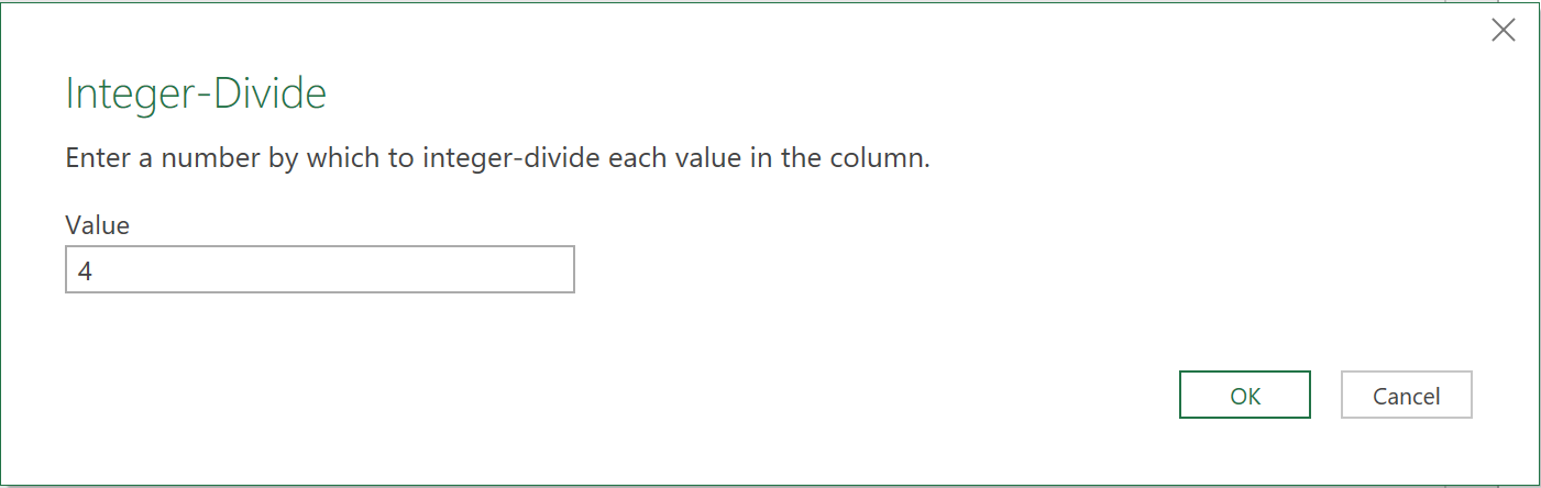
- Choose to divide by 4 ➔ click OK
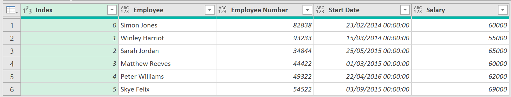
The index column should now look as follows:
3. Pivot the Data
Now, the data is ready to be pivoted
- Select Column 1 ➔ click the ‘Pivot Column’ icon under the ‘Transform’ tab
- Choose Column 2 as the Values column
- Under Advanced options, choose ‘Don’t Aggregate’
The data will now pivot properly, and look as follows:
4. Load the data to Excel
- Finally, remove the Index column as it is now no longer needed
- Close and Load the query to Excel
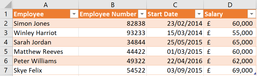
After some formatting, you should have a table that looks like this, showing the data in the desired layout!
Feedback
Submit and view feedback