Grouping Tables (to show row detail)

Overview

In this article, we understand a technique for Grouping Tables, but at the same time showing some of the underlying row detail - which is something not possible with standard Pivot Tables.

Grouping Tables, but also showing underlying row detail

Excel PivotTables function well when you need to summarise data. If a field is numeric, cells will be added; if a field is non-numeric in nature, items will be counted.

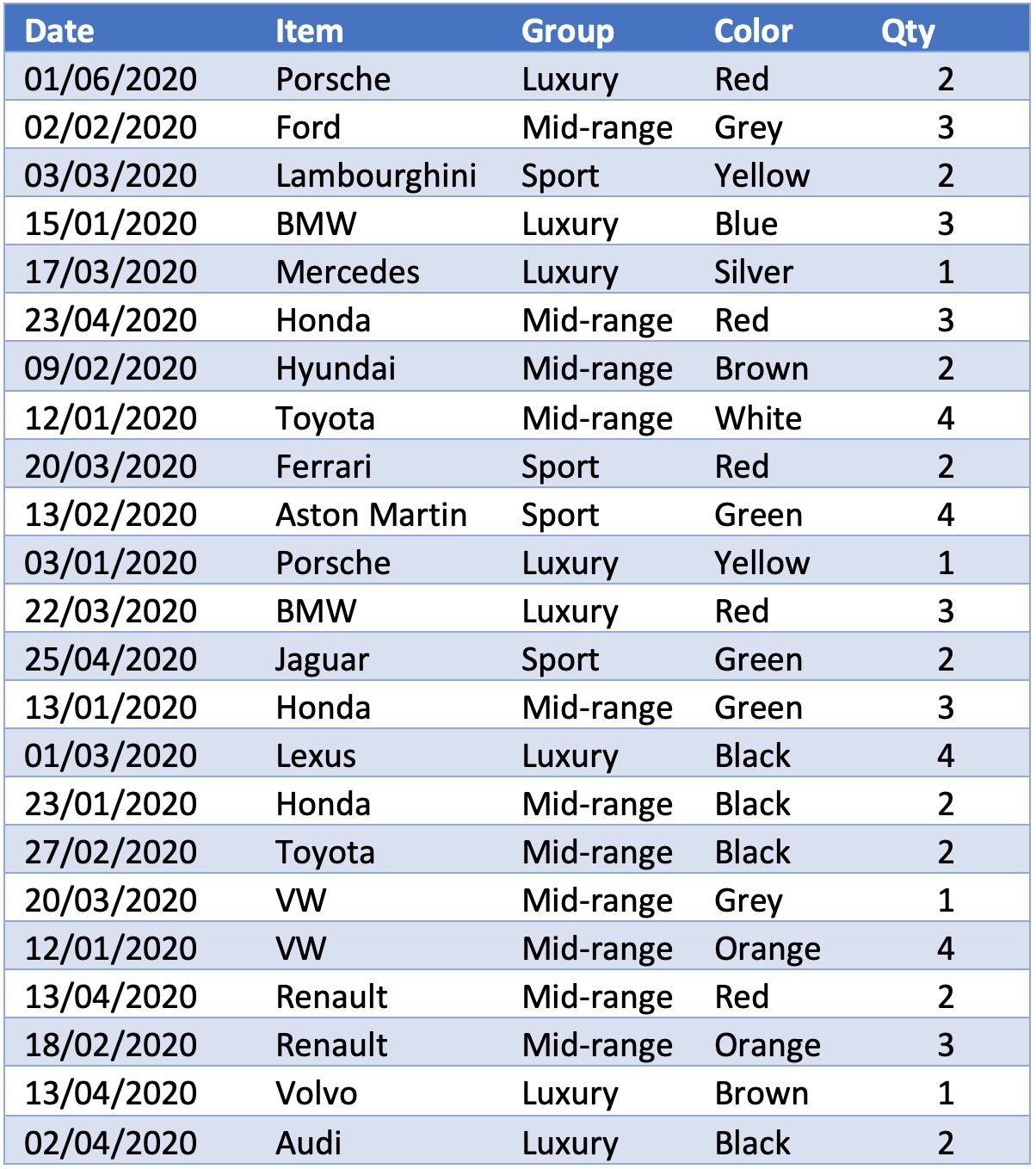
The Excel Table below shows an example dataset with both numeric and text fields.

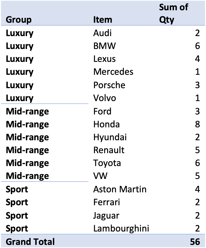
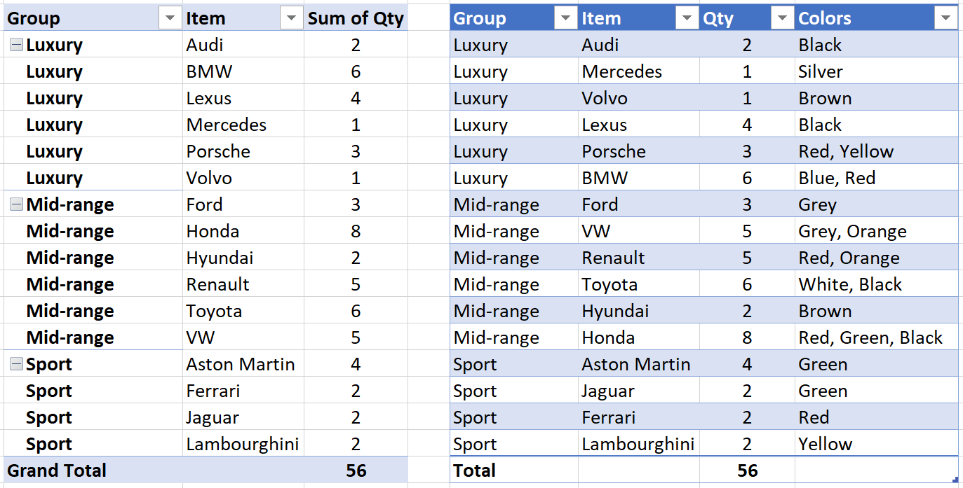
The same data can be summarised using a standard Pivot Table, as shown below:

Now, if you double click on VW, a new sheet will appear showing the underlying row detail that make up the Quantity of ‘5’. As shown below, there are 2 rows.

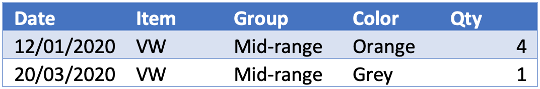
This data, however, cannot be summarised in the Pivot Table itself (for example, the colors, Orange, and Grey are not shown in the above Pivot Table). Below we show how this can be done with Power Query instead.

Steps

1. Create a new Query, and Group by the columns ‘Item’ and ‘Group’

To start, create a new Query from the original data-source.

• Click anywhere in the Data Source Table
• On the ‘Data’ tab, in Excel, select the ‘From Table/Range’ icon.

The Query Editor will then appear. In the Query Editor:

• Remove the Date column
• Then, highlight the ‘Item’ and ‘Group’ columns (press Shift to multi-select), and select the ‘Group By’ icon under the Transform tab.
• Configure the settings as shown below:

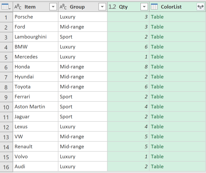
The Query editor should now look like this, with a Table object added to each row:

2. Add a Custom Column to show the row detail

Now, add a custom column, using the following ‘M’ code:

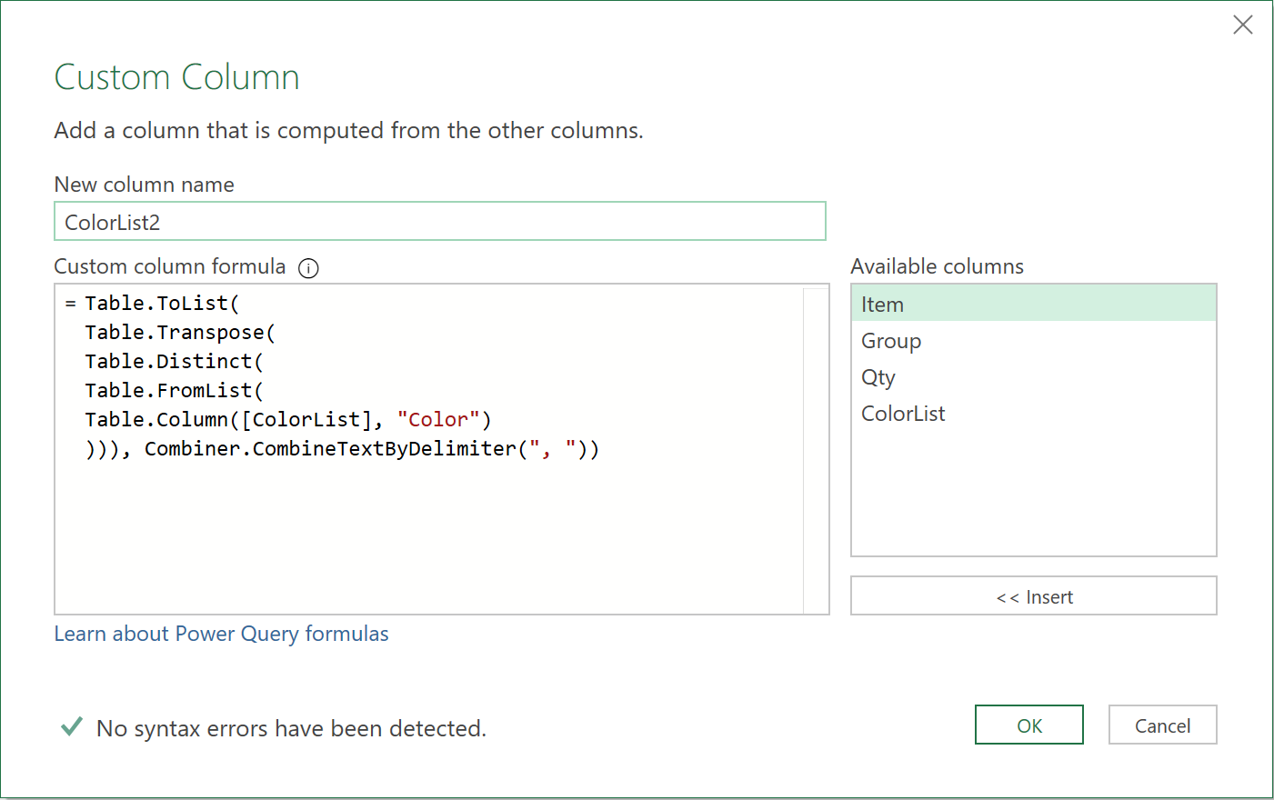
The formula:

• Takes the values from the column called ‘color’, from each Table object, and turns them into a list of lists
• Turns the list of lists into a series of Tables
• Removes any duplicate values from each Table
• Transposes each Table, turning rows into columns, and columns into rows
• Turns each transposed table back into a list of lists, concatenating each item with a “, “ delimiter

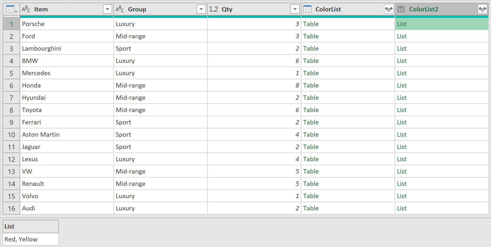
The Query Editor will now show a new column, like this, returning a List object to each row:

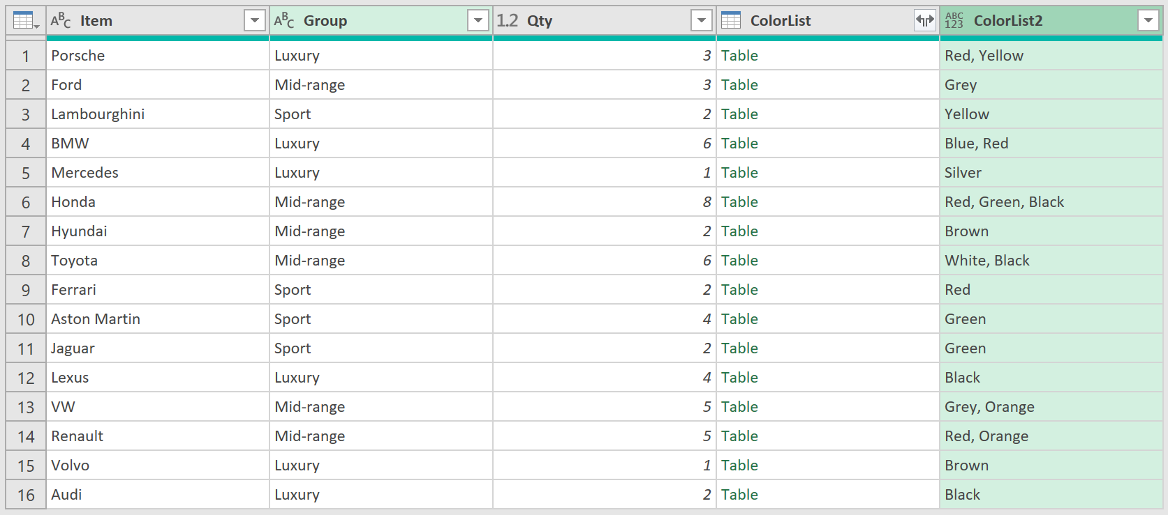
Click on the Expand Icon, and then ‘Expand to New Rows’ options. This will change the List objects in this column to show the underlying row detail, of the ‘color’ field.

After reordering, renaming, and deleting any unneeded columns, click on ‘Close and Load To’ to load the query to a worksheet in Excel.

As shown below, the Power Query output is identical to the Pivot Table, except that the extra level of color detail, as we had wanted, is also included!