Grouping Tables (to show rankings)

Overview

In this article, we understand a technique for Grouping Tables, so that records can also be ranked, according to some criteria.

Scenario

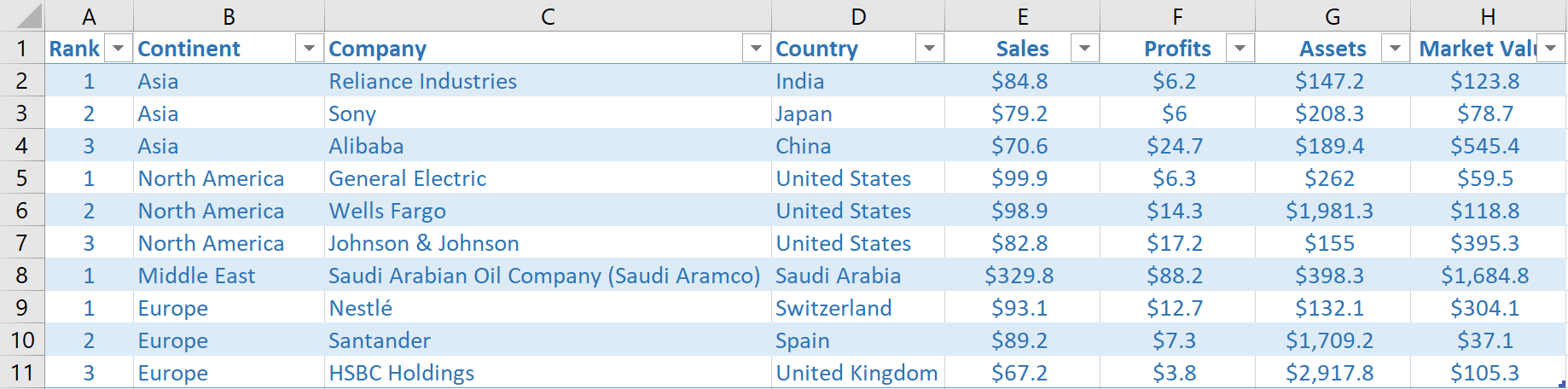
Let’s suppose we have data that looks like this, which shows the top global companies, by their main financial metrics.

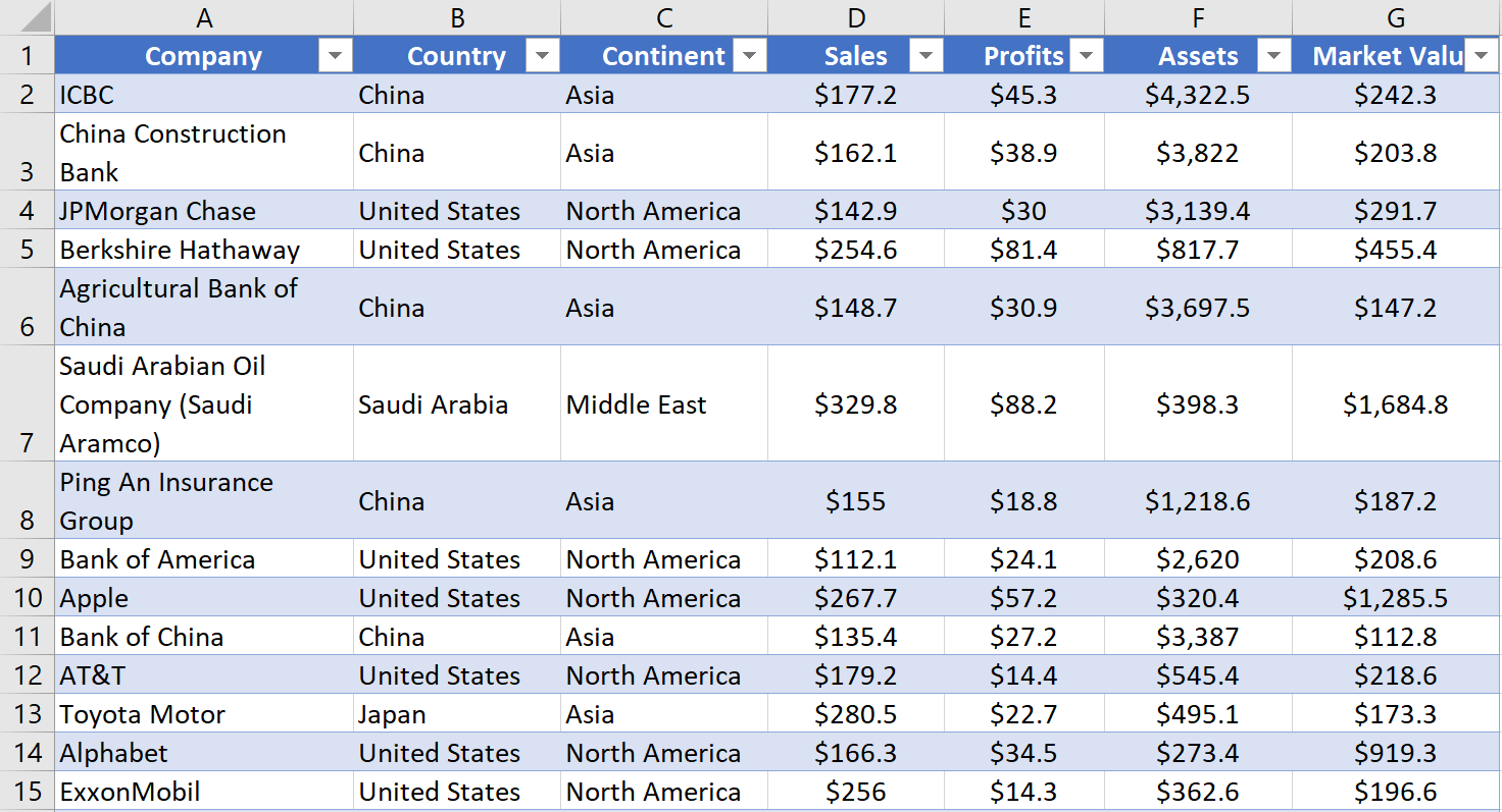
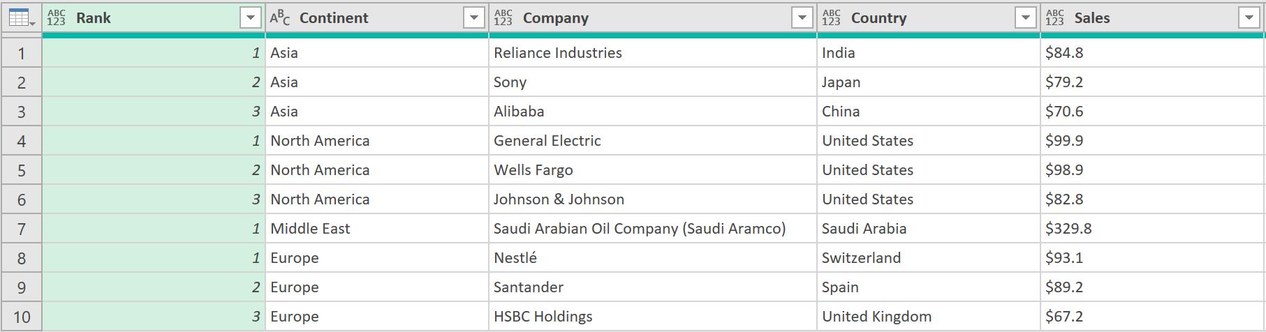
We wish to summarise this data, showing only the top 3 companies by continent, ordered in descending order. The following explains how to achieve this, using various functions.

Steps

1. Group the Data in Power Query

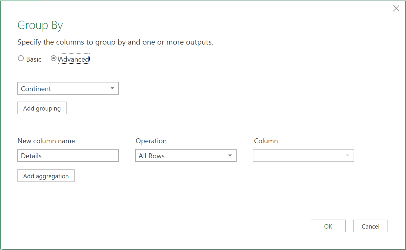
• Load the Data into Power Query, and click on the Group By icon, under the Transform tab
• Apply the following settings in the Group By dialogue window (grouping by ‘Continent’, adding a new column, with the operation ‘All Rows’

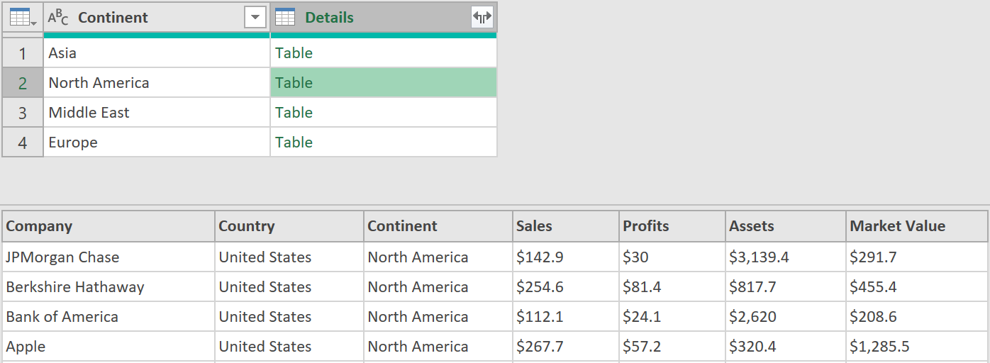
• The query should look like this, with a Table Object loaded to each row (each Table Object, when clicked on, should show all the rows that form part of each Continent).

2. Add Custom Columns

• Now, add a custom column, with the following formula

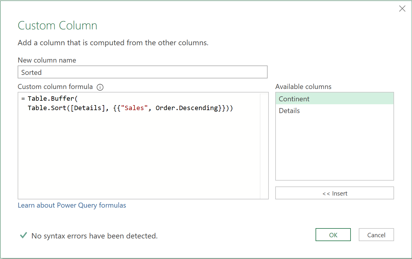
This will order the rows, by ‘Sale’ in each Table object. (The ‘Buffer function’ is here to ensure the data gets loaded into memory, and is sorted in the correct descending order)

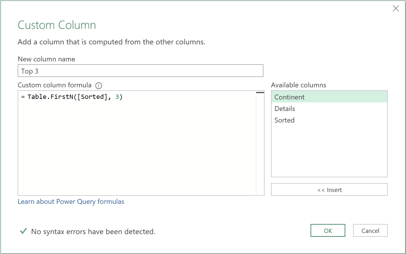
• Next, add another custom column, so that only the top 3 rows are kept, as follows:

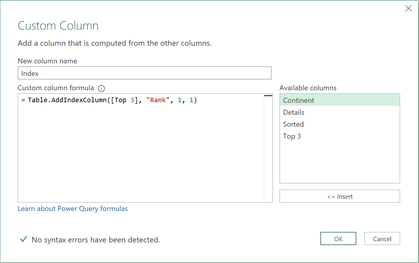
• Add a final custom column, to apply an Index to each Table object, as follows:

3. Expand the necessary fields

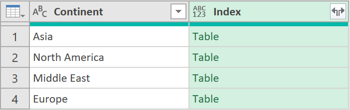
• Delete the columns, ‘Details’, ‘Sorted’, and ‘Top 3’ as they are now no longer needed, so you are only left with the ‘Continent’ and ‘Index’ columns, as shown here:

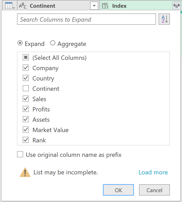
• From the ‘Index’ column, expand all fields (except the ‘Continent’ field, as it is already there), as shown here:

• After the fields have been expanded, bring the ‘Rank’ column, to the far left, so the query looks like this:

• Load the Query to Excel, by clicking on Close & Load.

The results should look as follow – a ranking of just the top 3 companies, by Continent, by their Annual Sales - just as we had originally wanted!