Pivoting on multiple measures

Overview

Sometimes, you may be given data in the below format, and wish to show it in a more pivoted form across multiple measures.

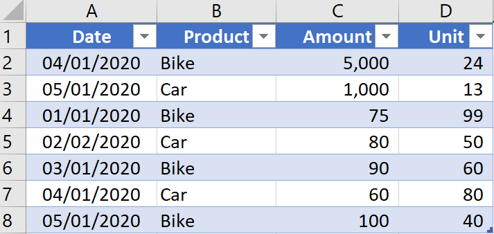
For example, with the above data, you might want to see the ‘sum of amount’ and ‘sum of unit’ measures, but separately for both Cars, and Bikes.

This article explains how you would do this.

Steps

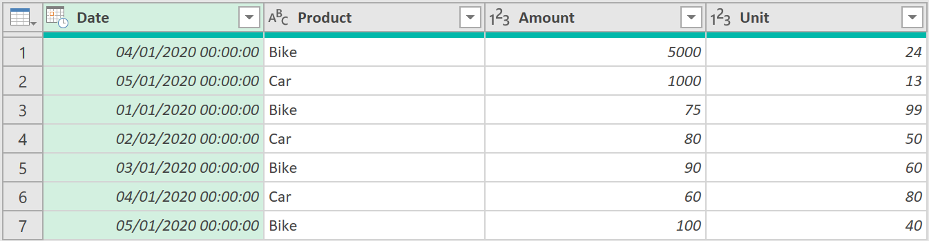
1. Load the data to power query

When loaded into the query editor, the data should look something like this:

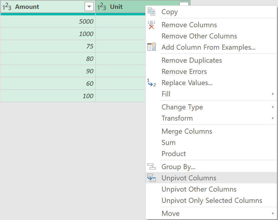
2. Unpivot the data

• Next, select the columns called ‘Amount’ and ‘Unit’
• Right-click, and select from the menu that appears, the ‘Unpivot Columns’ option

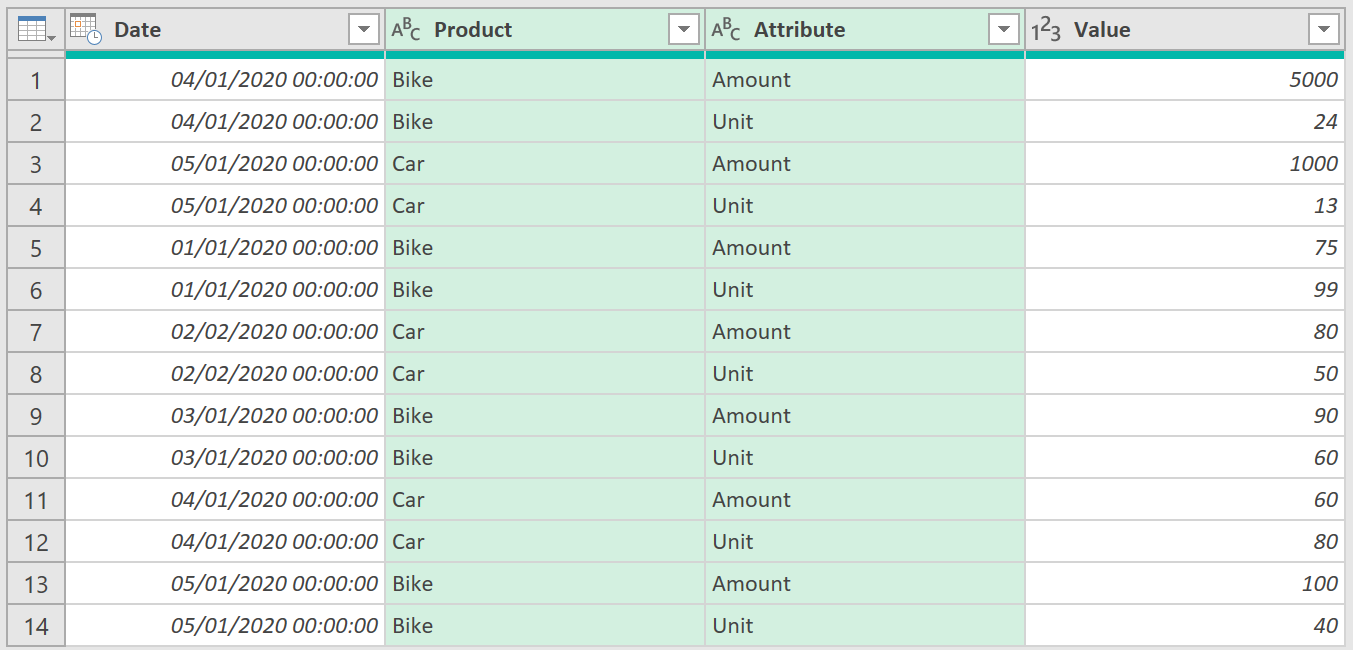
The data should now look something like this:

3. Merge columns

• Now select the columns ‘Product’ and ‘Attribute’, right-click, and choose the option Merge Columns

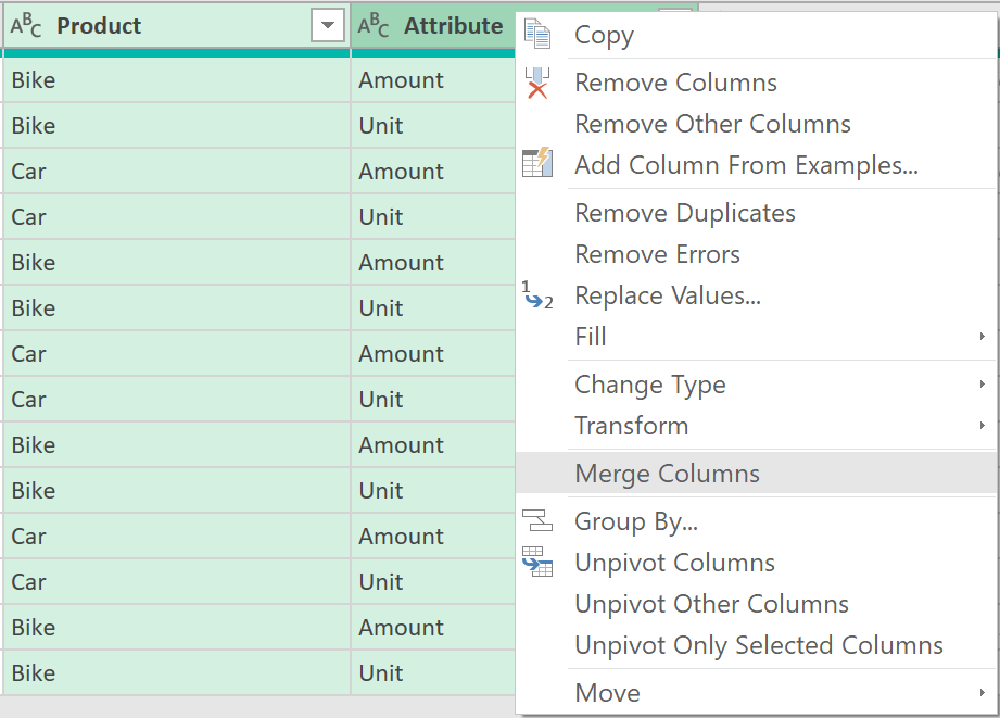
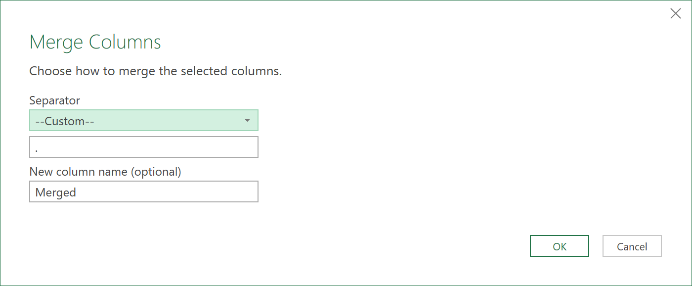
• Choose the custom separator ‘.’ as shown below:

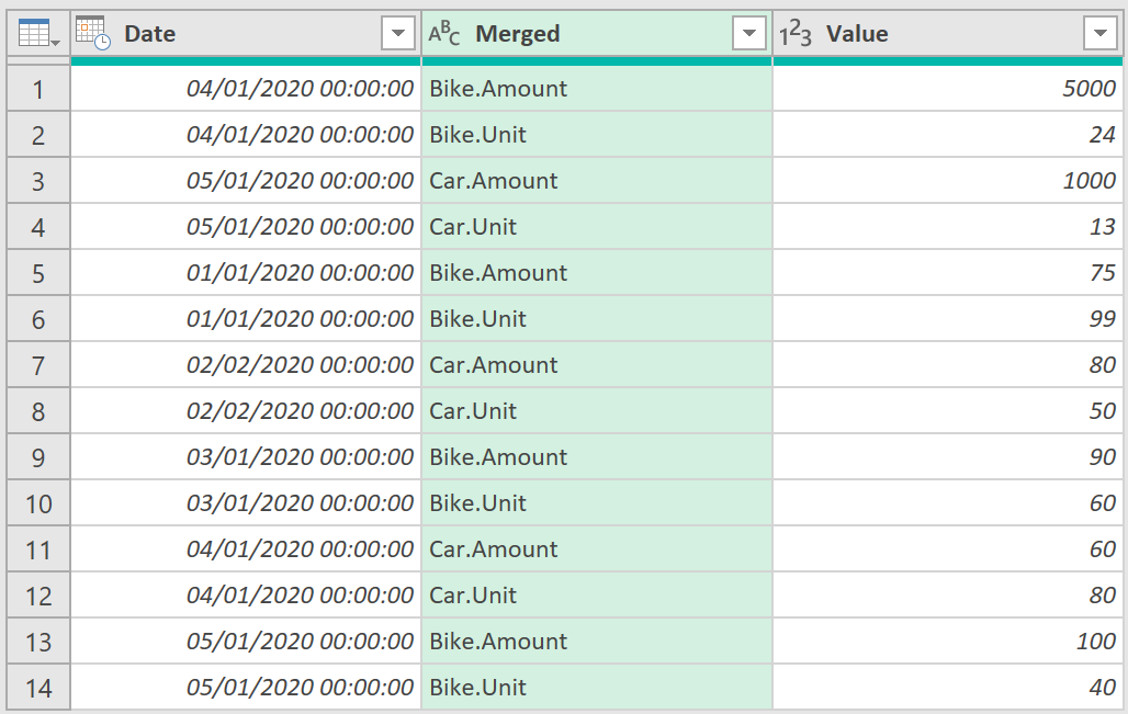
After merging the columns, the data should now look like this:

4. Pivot the data

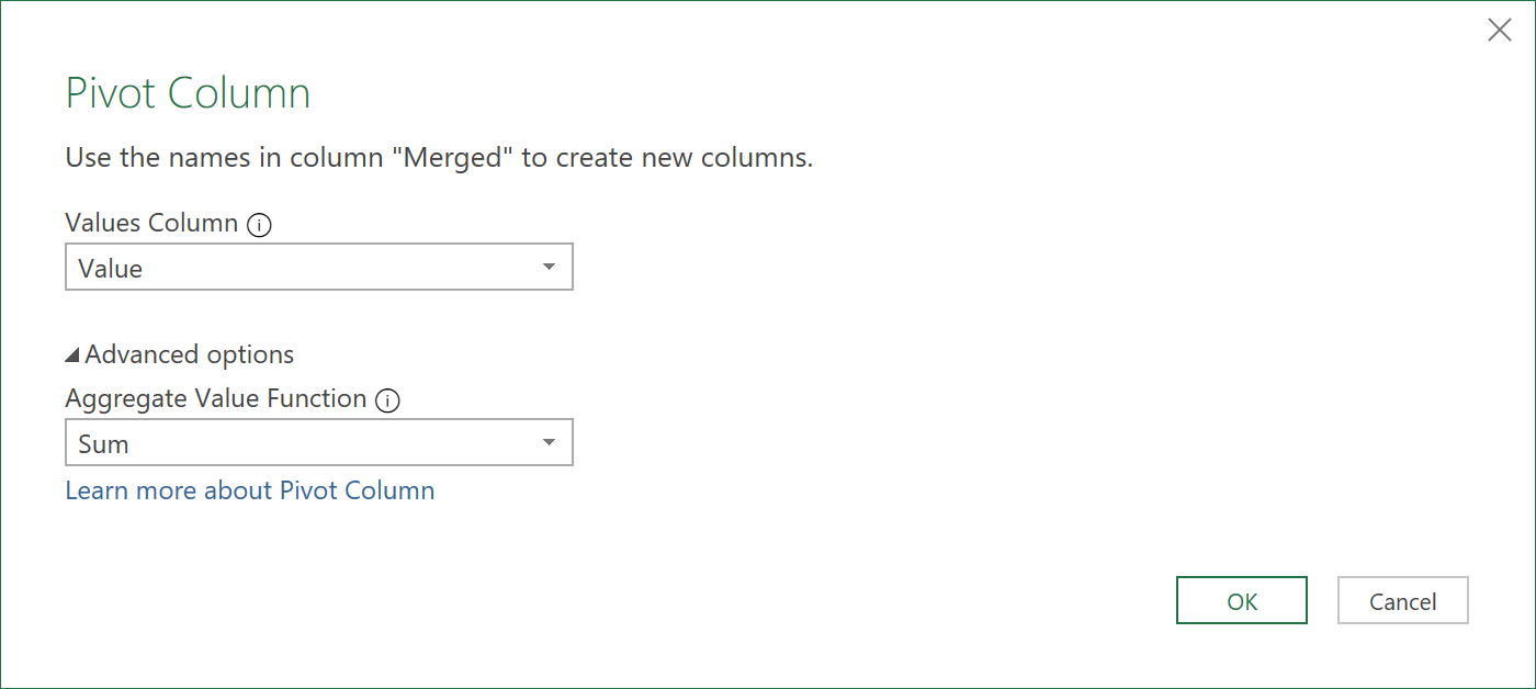
• Click on the column called ‘Merged’ and click on the ‘Pivot Column’ icon under the ‘Transform’ tab
• Use the following settings in the next window that appears:

• Change the ‘Data’ type of the ‘Date’ column to type ‘Date’. The data should now look as follows:

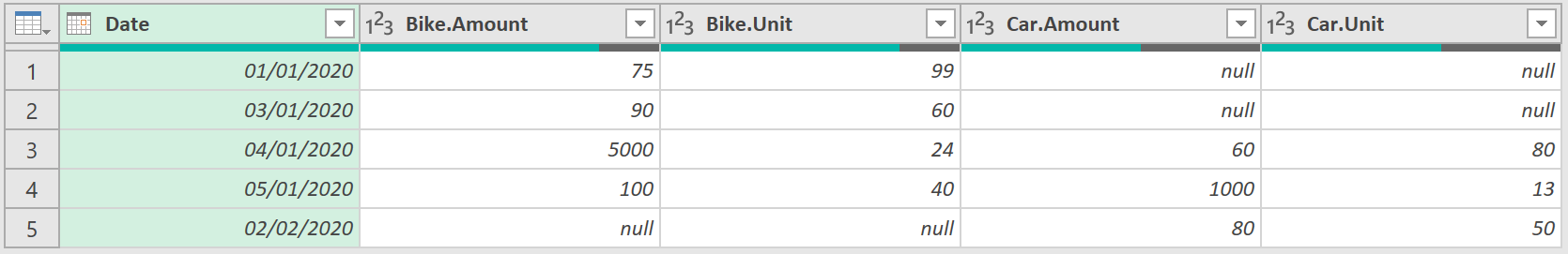
The data is now in the pivoted form we had originally wanted!

• Click Close & Load to load the results to Excel