The Challenge! - combining revenue files

The Challenge!

In this article, we bring together different elements, to overcome a particular challenge:

You have just been appointed Chief Information Officer of Galactic Ventures Limited, but last weekend, the company’s data warehouse was hit massive cyber-attack, and you have been called in to save the day!

The challenge is to try to re-construct a new report from the company’s old revenue data (what is left of it anyway…)

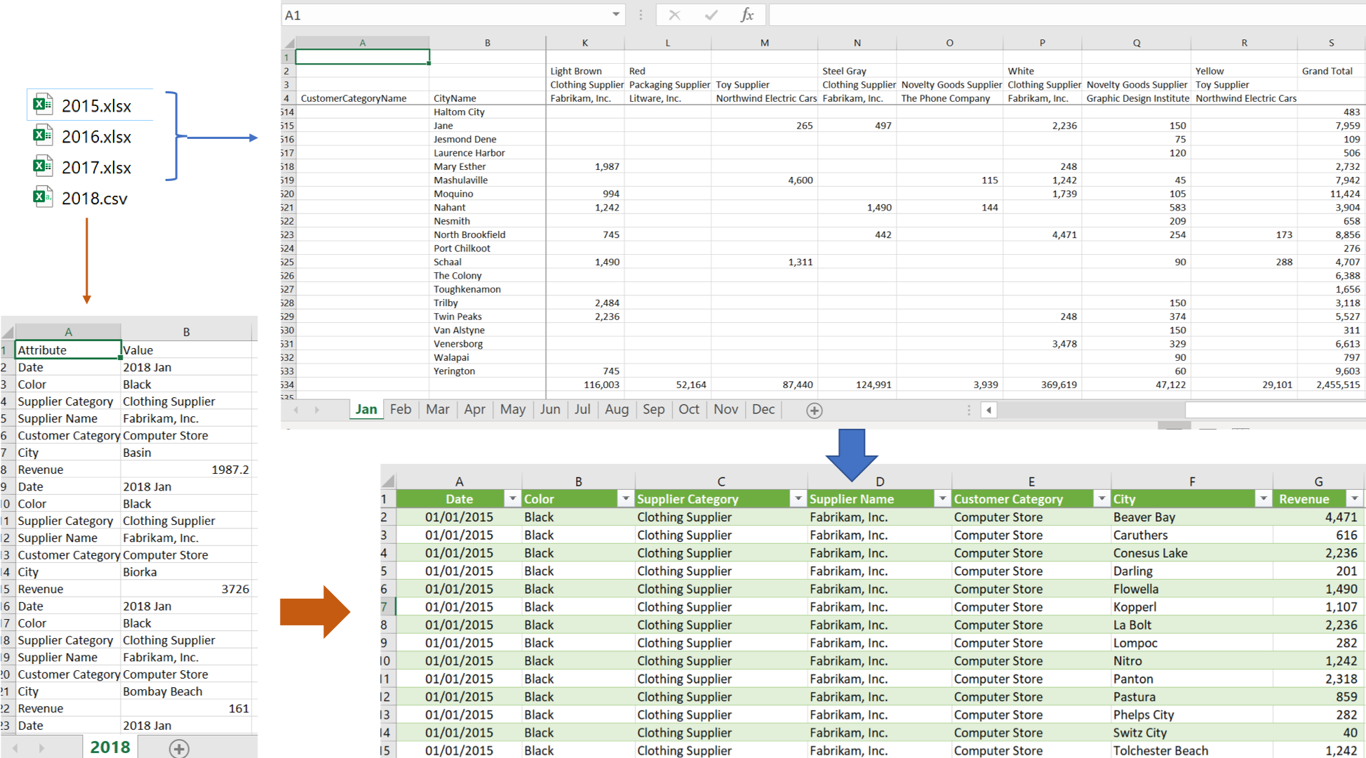
Luckily, your predecessor did some record-keeping, and kept all the revenue reports for the years 2015 to 2017, in three Excel workbooks. Each workbook has 12 worksheets, one for each month of the year (i.e. Jan, Feb, Mar…. Dec).

The 2018 revenue file however was kept in a different CSV format. (God knows why, but, for now, just accept that it was!)

The goal is now to try and combine data from all 36 worksheets for the years 2015 to 2017 (data currently stored in pivoted data table format) - together with the 2018 revenue data (data currently in multi-line record format), into one single table, like the one shown below:

The problem can be solved by breaking it down into three parts. The solution to each is laid out in the follow sections.

Combining xlsx files

To start with, the three revenue files that are in the same format (2015 to 2017):

1. Load the data

• Open a Blank Query in Excel. Then, in Excel, select the Data tab, then ‘Get Data’, then ‘From File’, then ‘From Folder’

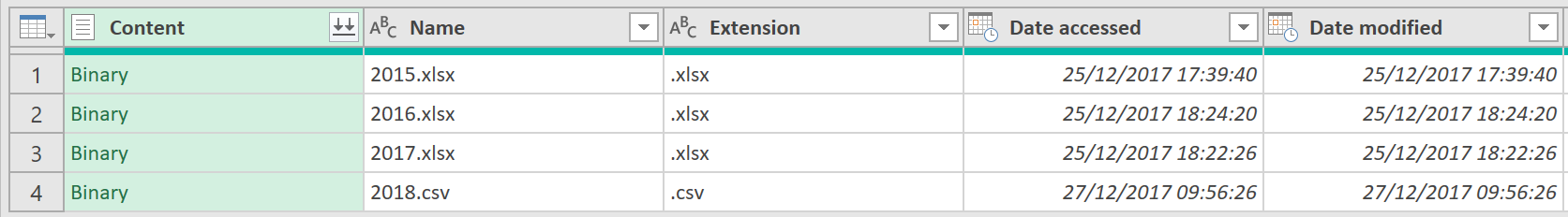
• Select the Folder where the old Revenue files are kept, as shown here:

• Filter out the 2018.csv file, which has a different format to the other files.

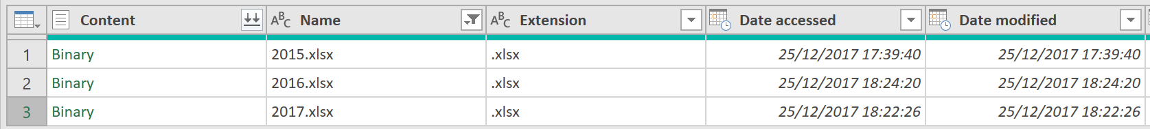
• Rename the Query to “Revenues”

2. Combine Files

• Next, click on the “Content” column, and then click on the “Combine Files” icon on the Home tab.

• In the Combine Files dialog box that appears, right click on “Sample File Parameter1”, and select Edit, as shown below:

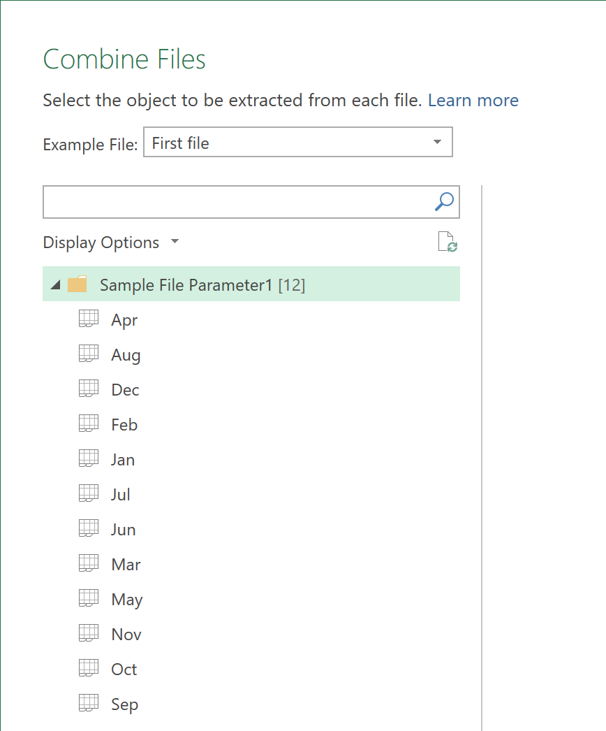
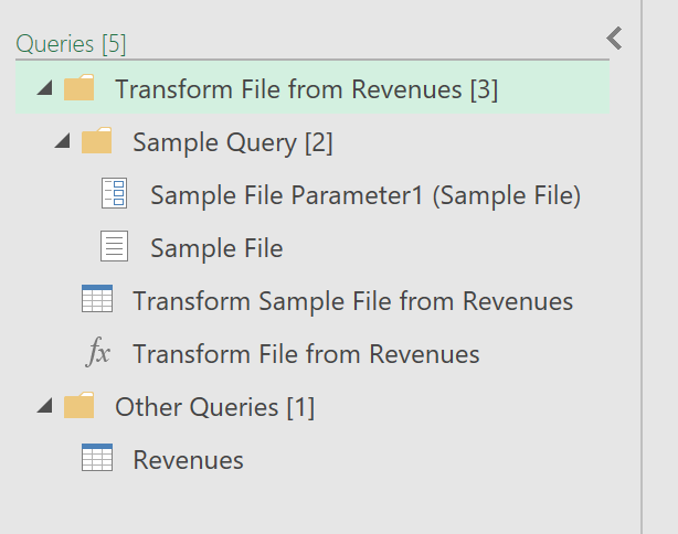
This step is quite important as it will auto-generate a series of other queries, that will show up on the left-hand pane, as shown below. Do not become too concerned with why they are there, and what they do, just know that because you are pulling data from a folder, instead of a single file – they are needed.

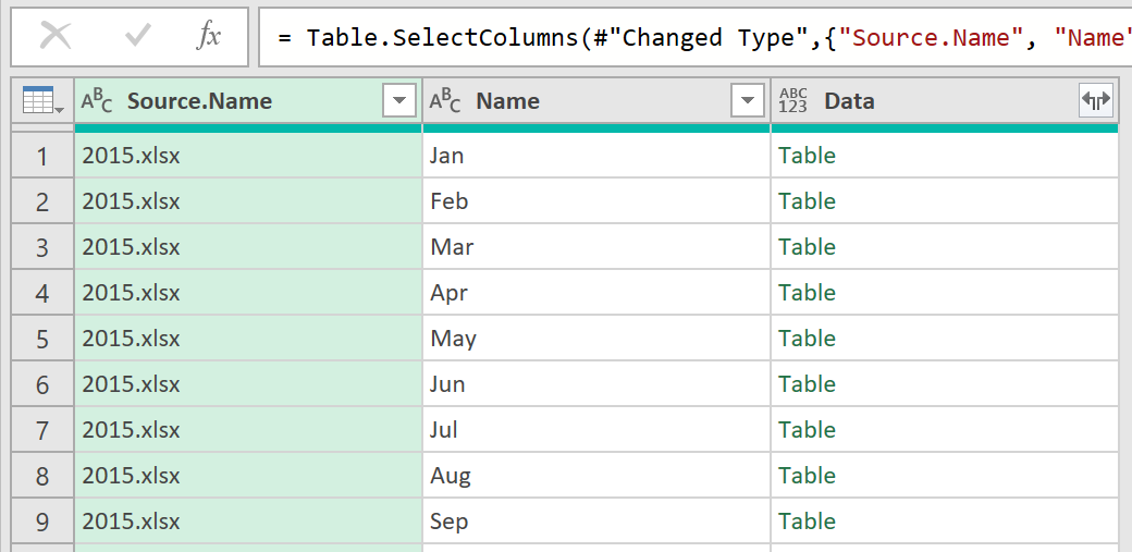
• With the necessary queries generated, click back to the “Revenues” Query, and remove all but the first three columns, as shown below:

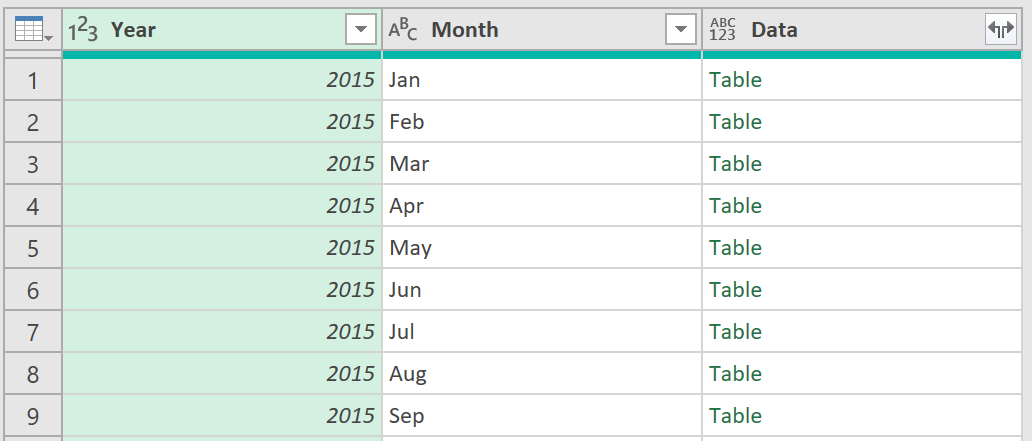
• Now rename the first two columns to “Year”, and “Month” respectively, as shown:

3. Create function 1

• Next, create a function that will clean up the data from each of the 36 Tables (there are 12 in each file).

The function you create should automatically remove the 1st row, which is not needed, the last column (which is the Grand Total column), which is not needed, and then the last row (which is the Grant Total row), which is also not needed.

• Create the function as follows, by creating a Blank Query:

fnCleanSummarizedTable

(inputTable) =>
let
    SkipFirstRow = Table.Skip(inputTable, 1),
NoGrandTotalColumn = Table.RemoveColumns(SkipFirstRow, { List.Last(Table.ColumnNames(SkipFirstRow)) } ),
    Result = Table.RemoveLastN(NoGrandTotalColumn, 1)
in
    Result

The function should:

• Skip the first row
• Delete the last column
• Delete the bottom most row

Now, include the following Applied Step:

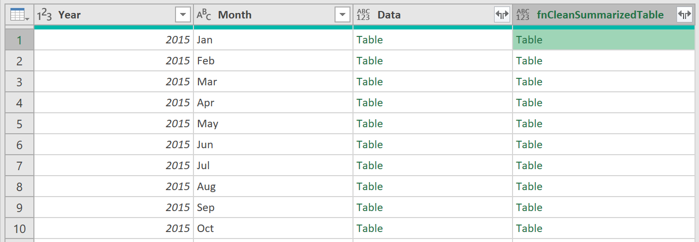
= Table.AddColumn(#"Renamed Columns", "fnCleanSummarizedTable", each fnCleanSummarizedTable([Data]))

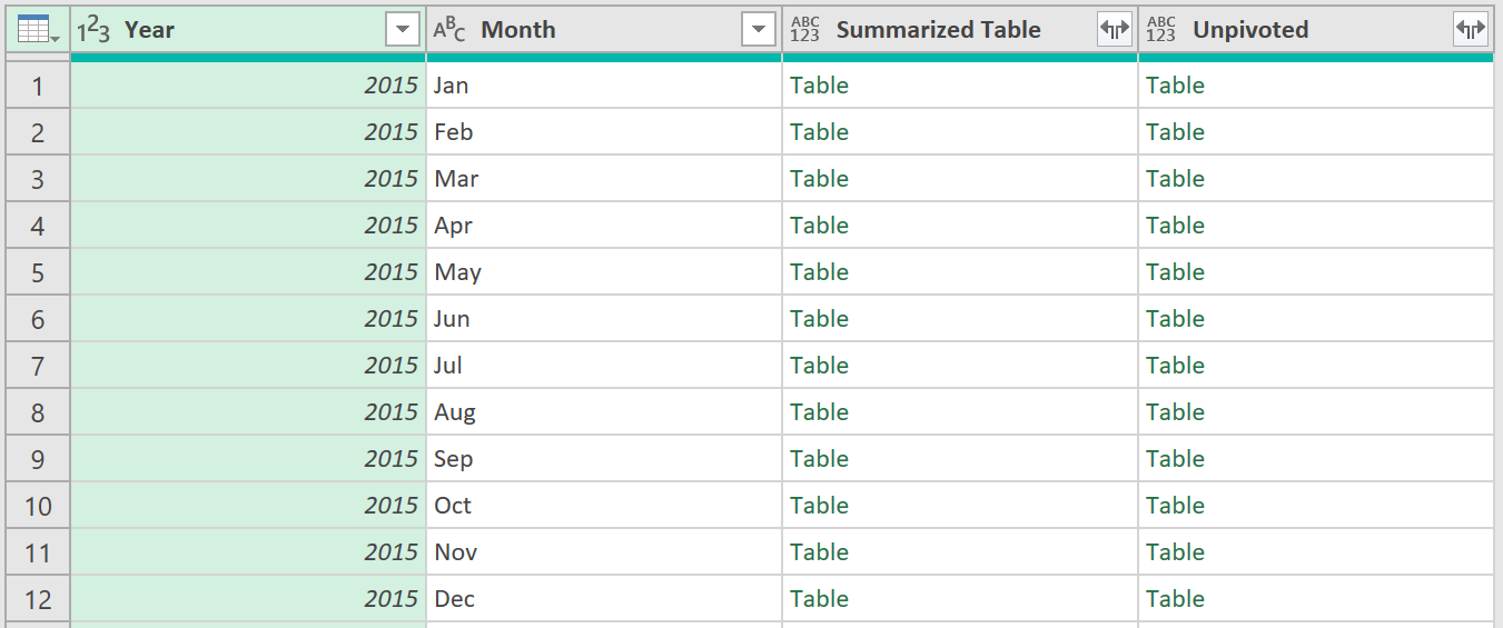
A new column should appear:

• Finally, rename the column to “Summarized Table”, and remove the column called “Data”, which is now no longer needed.

4. Create function 2

• Create another function that will take the data from these Summarized Table’s and unpivot their content.

Use the following code:

fnUnpivotSummarizedTable

let
    Source = (Source, RowFields, ColumnFields, ValueField)=>
let
    #"Filled Down" = Table.FillDown(Source, List.FirstN(Table.ColumnNames(Source), List.Count(RowFields) - 1)),
    #"Merged Columns" = Table.CombineColumns(#"Filled Down", List.FirstN(Table.ColumnNames(#"Filled Down"), List.Count(RowFields)), Combiner.CombineTextByDelimiter(":", QuoteStyle.None),"Merged"),
    #"Transposed Table" = Table.Transpose(#"Merged Columns"),
    #"Filled Down1" = Table.FillDown(#"Transposed Table",List.FirstN(Table.ColumnNames(#"Transposed Table"), List.Count(ColumnFields)-1)),
    #"Promoted Headers" = Table.PromoteHeaders(#"Filled Down1", [PromoteAllScalars=true]),
    #"Unpivoted Other Columns" = Table.UnpivotOtherColumns(#"Promoted Headers",List.FirstN(Table.ColumnNames(#"Promoted Headers"), List.Count(ColumnFields)) , "Attribute", ValueField),
    #"Split Column by Delimiter" = Table.SplitColumn(#"Unpivoted Other Columns", "Attribute", Splitter.SplitTextByDelimiter(":", QuoteStyle.Csv), RowFields),
    #"Renamed Columns" = Table.RenameColumns(#"Split Column by Delimiter", List.Zip({List.FirstN(Table.ColumnNames(#"Split Column by Delimiter"), List.Count(ColumnFields)), ColumnFields})),
    #"Changed Type" = Table.TransformColumnTypes(#"Renamed Columns",{{ValueField, type number}})
in
    #"Changed Type"
in
    Source

The function takes in four arguments. (Refer to this article on Creating a Generalisable function, for more details on how this function works)

• Now, call the function by adding the following Applied Step:

= Table.AddColumn(#"Removed Columns", "Unpivoted", each FnUnpivotSummarizedTable([Summarized Table], {"Customer Category", "City"}, {"Color", "Supplier Category", "Supplier Name"}, "Revenue"))

The query should now look as follows:

• Remove the “Summarized Table” column, as this is now no longer needed.

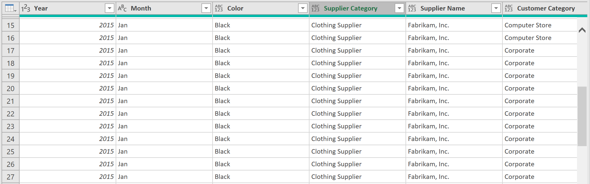
• Finally, expand the Unpivoted Column, deselecting “Use Original Column Name As Prefix” option, and then click OK.

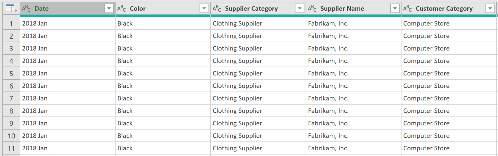
The data should now be in the format needed.

UNFORTUNATELY, THOUGH, THIS IS ONLY…

…HALF THE BATTLE!

You next need to transform the 2018 Revenue data – which was in a different format.

Loading csv file

• To transform the 2018.csv file into the right shape, in the Power Query Editor, select “New Source”, and Choose File, and then Text/CSV.

1. Load the data

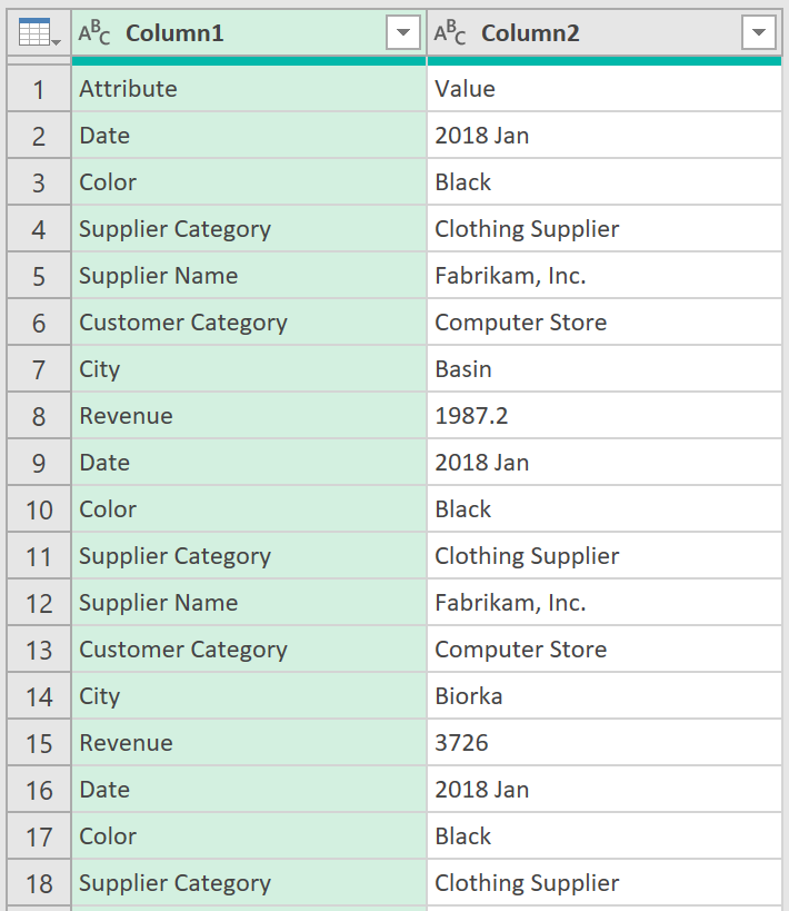
• Import the CSV file (as explained above), and rename the query to “2018 Revenues”, so that you see something like the below:

• On the Transform Tab, select “Use First Row As Headers”

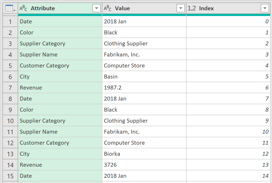
2. Add an index column

• Then, on the Add Column Tab, select Index Column, like so:

3. Create a conditional column

• Now, create a Conditional Column, with the following parameters:

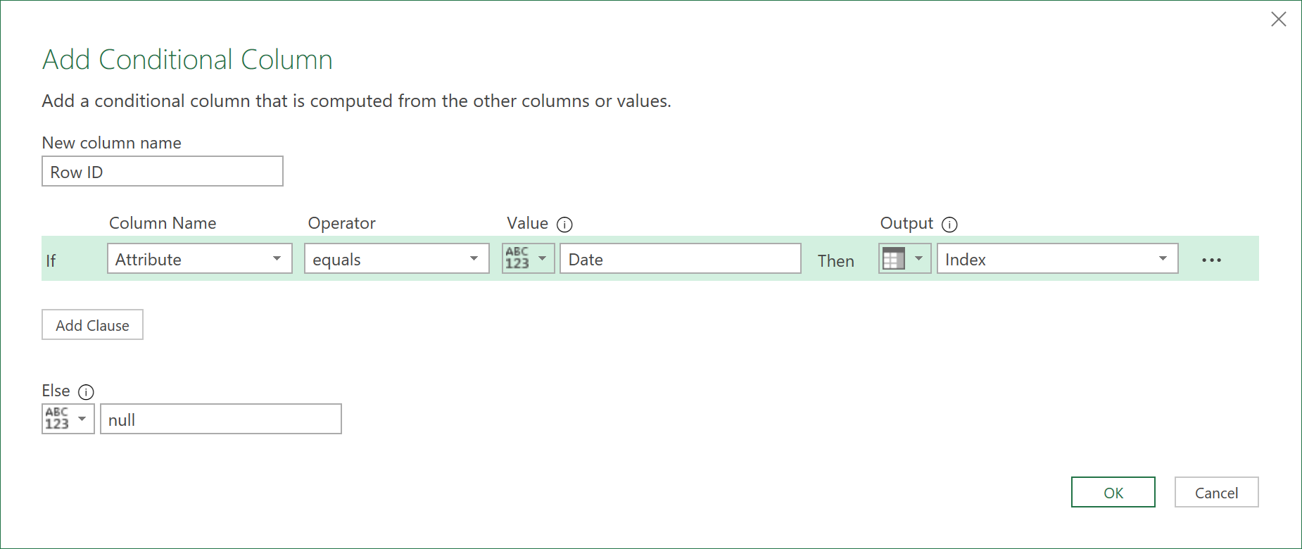
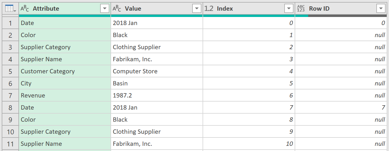
The data should look like this:

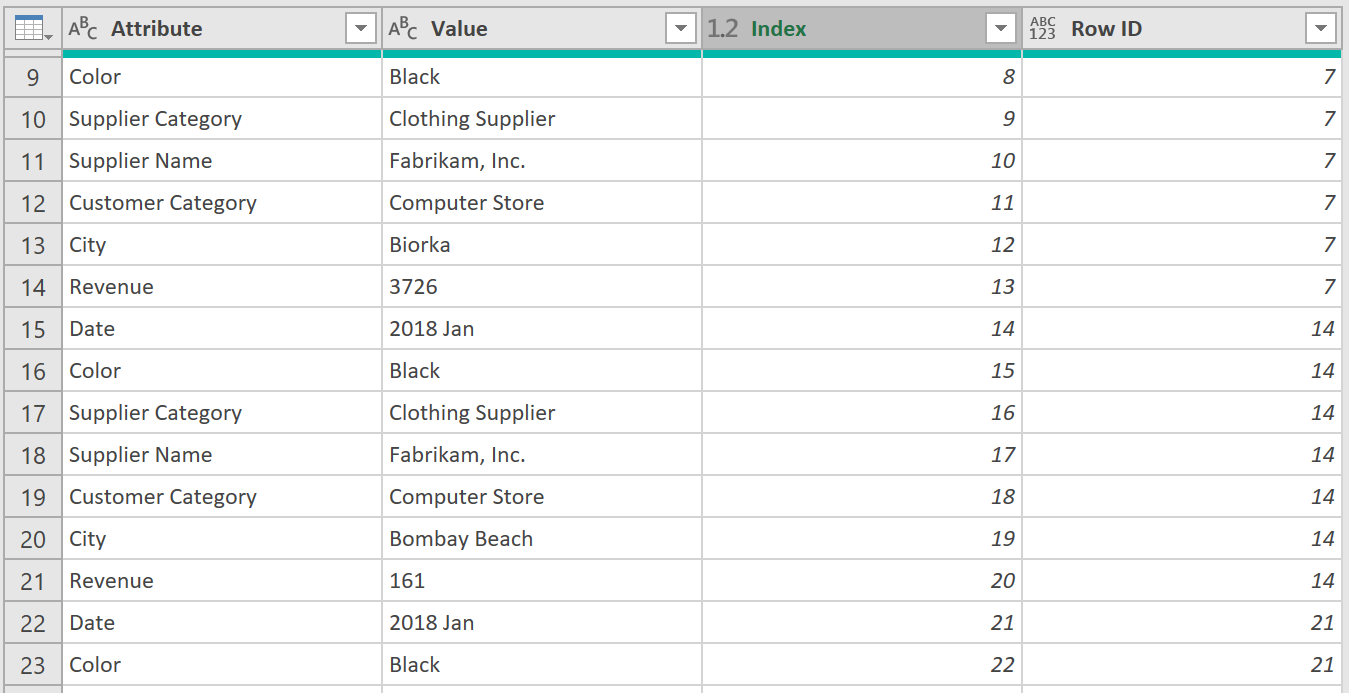
4. Fill down the data

• Now, select the ‘Row ID’ column, and then on the Transform Tab, select Fill, Down, so the data looks like this:

• Delete the Index column, as it is no longer needed.

5. Pivot the data

• Now, select the “Attribute” Column, and on the Transform Tab, select Pivot Column.

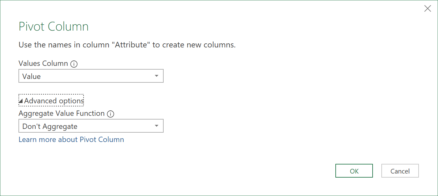
The data should now look like this:

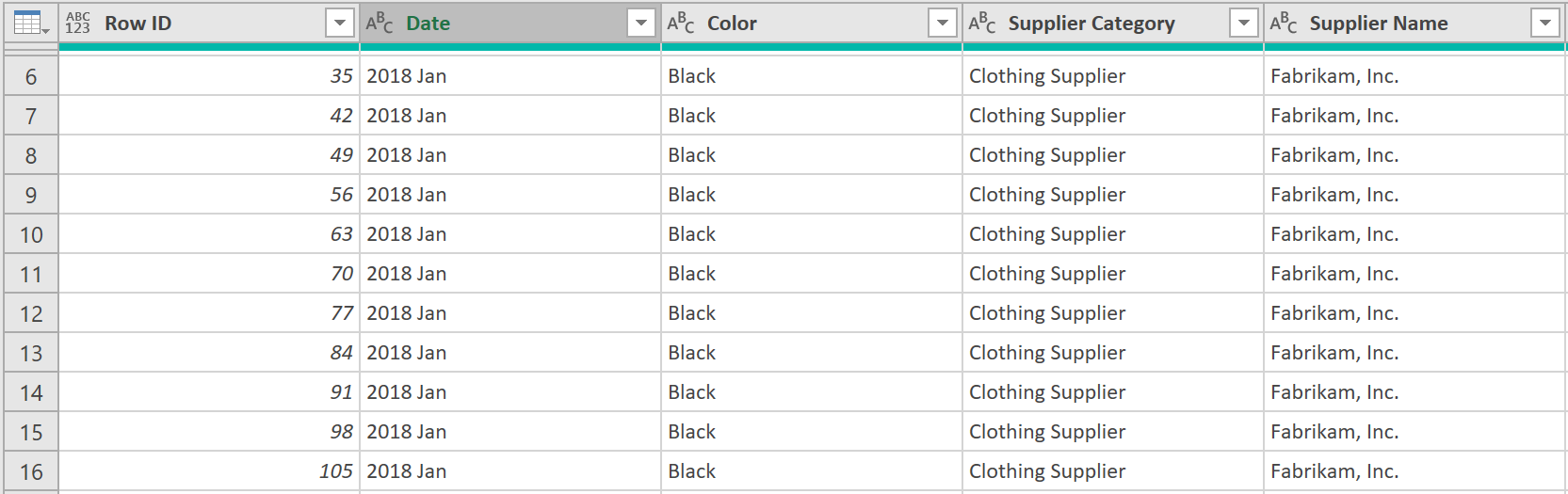
• Now, remove the Row ID column, as it is not needed:

WE ARE NOW 5/6ths OF THE WAY THERE!

The final, last step is to append both queries together into one final dataset.

Combining all files

Now you need to append the two earlier datasets together to form one whole.

1. Merge Columns

• Go back, and select the “Revenues” query, and select the columns called “Year” and “Month”, and then on the Transform Tab, select Merge Columns.

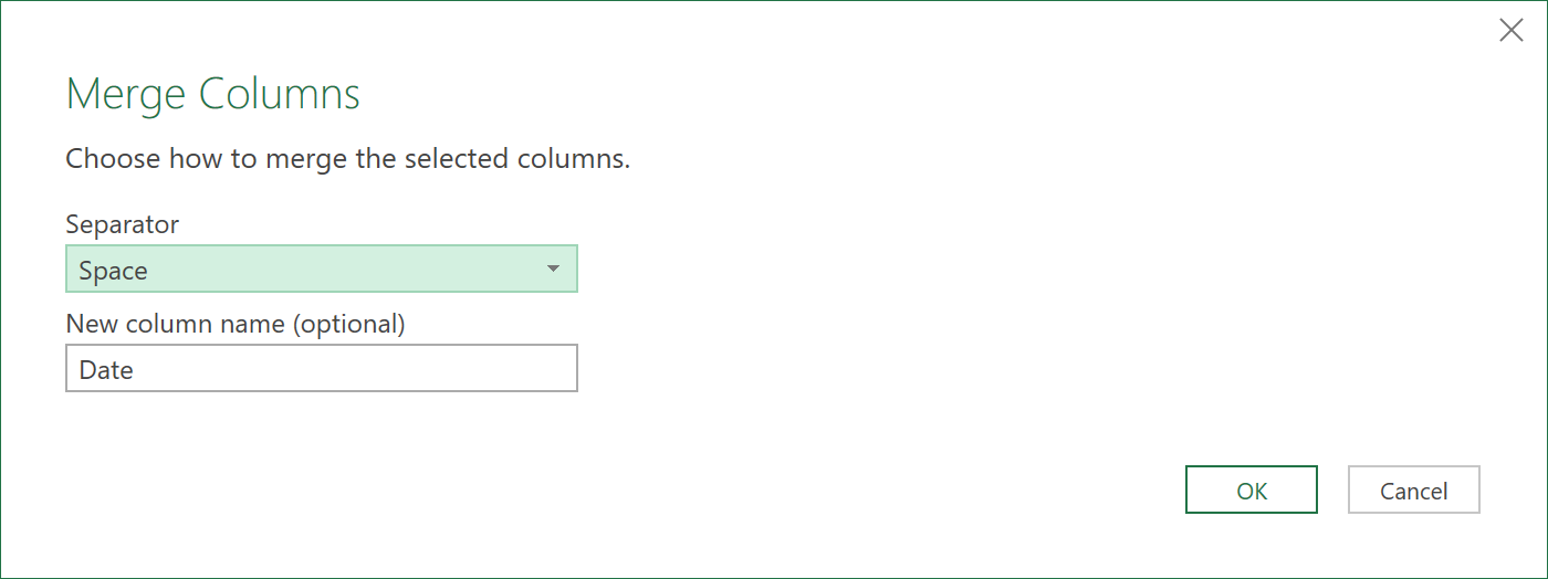
• In the Merge Columns Dialog Box that appears, select Space as the Delimiter, and enter Date in the New Column Name box. Then click OK.

2. Append Queries

• Next, on the Home Tab, select Append Queries. In the Append Dialog box that appears, set the Table to Append “2018 Revenues”, and then click OK.

3. Set Data types

• Change the Data Type of the columns, “Revenue”, and “Date”, to “Currency”, and “Date” respectively.

4. Close & load

• Finally, load the final query, by clicking on “Close & Load”!

If all has gone according to plan, you should see this….

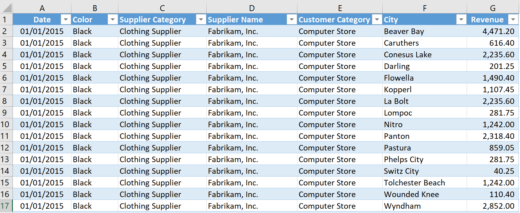
All the data, from 2015 to 2018, should now be in one Dataset! Congratulations!

GALATIC VENTURES LIMITED IS STILL IN BUSINESS!