
Preserving Context
Overview
Often mismatched silos of data need key contextual information stored elsewhere outside of the main data table (e.g. in the filename itself, the name of the worksheet, or typed in a cell at the top of a worksheet)
Combining tables without any context can risk giving meaningless results.
This article explains how you can dynamically detect and extract the correct “context” elements from your data, whilst ignoring the elements that are not needed.
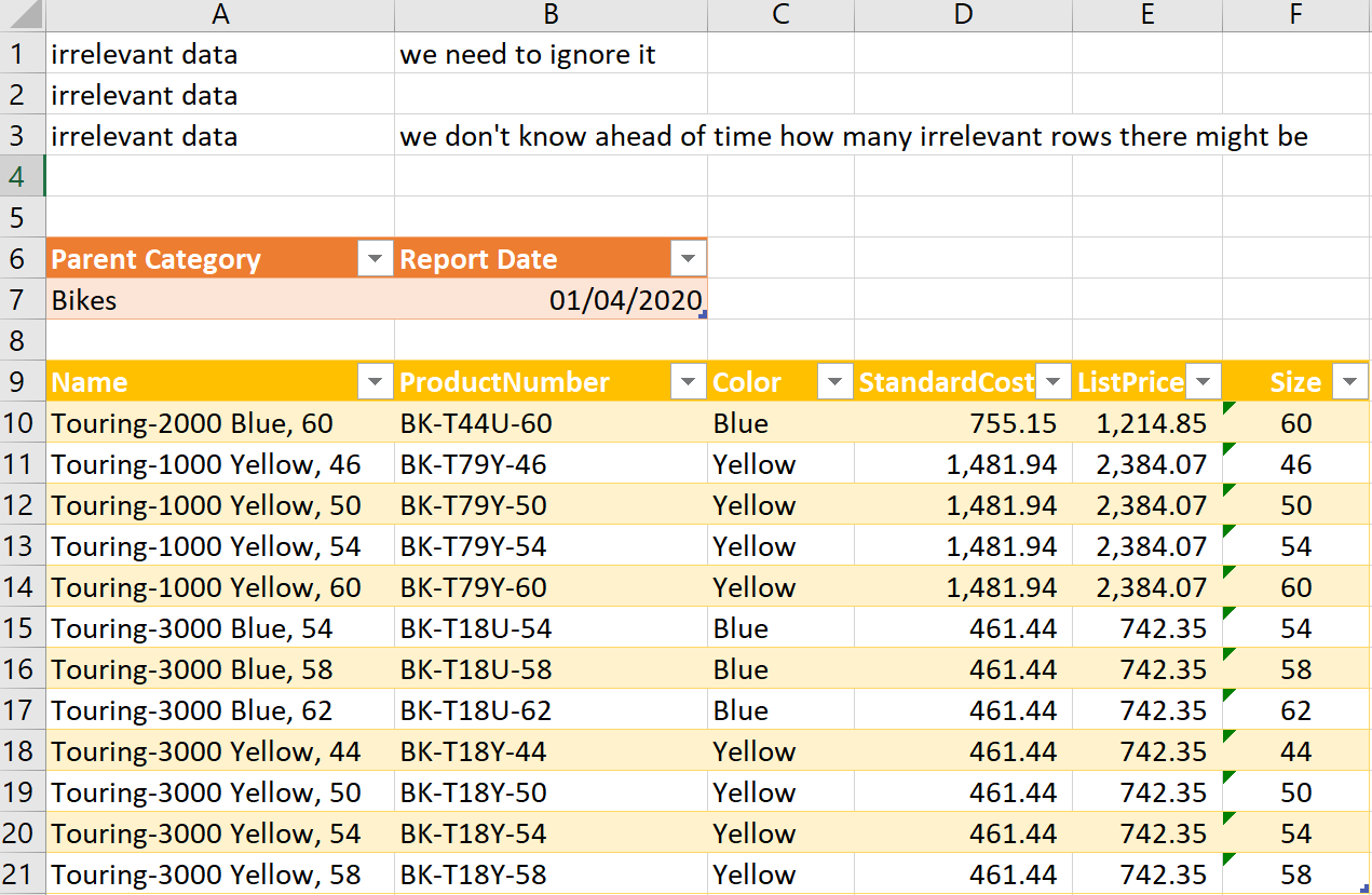
In the following example, contextual information is stored outside the table, at the top of the worksheet – (though the sheet also has a lot of irrelevant rows above it)
The technique described is especially useful when your data source includes multiple tables in the same file – each separated from its preceding table by a title line.
To correctly, and automatically extract the correct “context”, you should work through the following steps:
Steps
1. Load the data
- In Excel, go to ‘Get Data’, ‘From File’, ‘From WorkBook’.
- Choose the file called: Products.xlsx (which holds all the Product Parent Tables, stored across separate tabs).
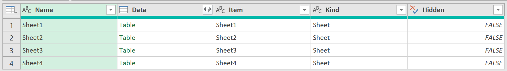
- Let the Query Editor load, so that it shows the 4 separate tabs:
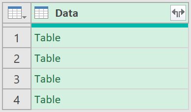
2. Clean the data
- Now, remove all meta-data columns, apart from the “Data” column. So, right-click on the “Data” column, and select the option to “Remove Other Columns”.
You should be left with just this:
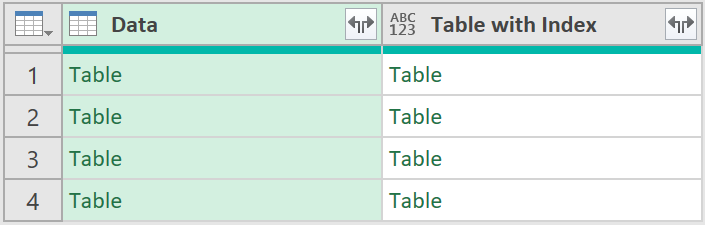
3. Add Index columns
- Next, add a custom step, with the following code, as shown below:
= Table.AddColumn(#"Removed Other Columns", "Table with Index", each Table.AddIndexColumn([Data], "Index", 0, 1))
The data should now look like this:
4. Add the row index of the context
- After this, add the following custom step, with the following code:
= Table.AddColumn(#"Custom1", "Row Index of Parent Category", each List.PositionOf([Data][Column1], "Parent Category"))
The data should look like this:
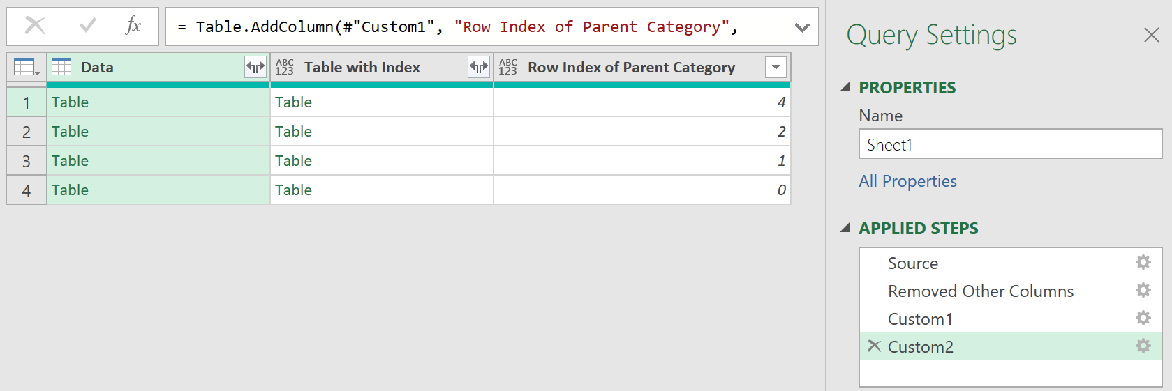
The line returns the row index where the field called, “Parent Category” is hardcoded. Each number represents the location of the “Parent Category” cell in a zero-based index.
The row index returned would vary for each Data Table, given the different number of irrelevant rows in each sheet.
5. Add context data
- Next, add the following line of code:
= Table.AddColumn(#"Added Custom1", "Parent Category", each [Data]{[Row Index of Parent Category] + 1}[Column1])
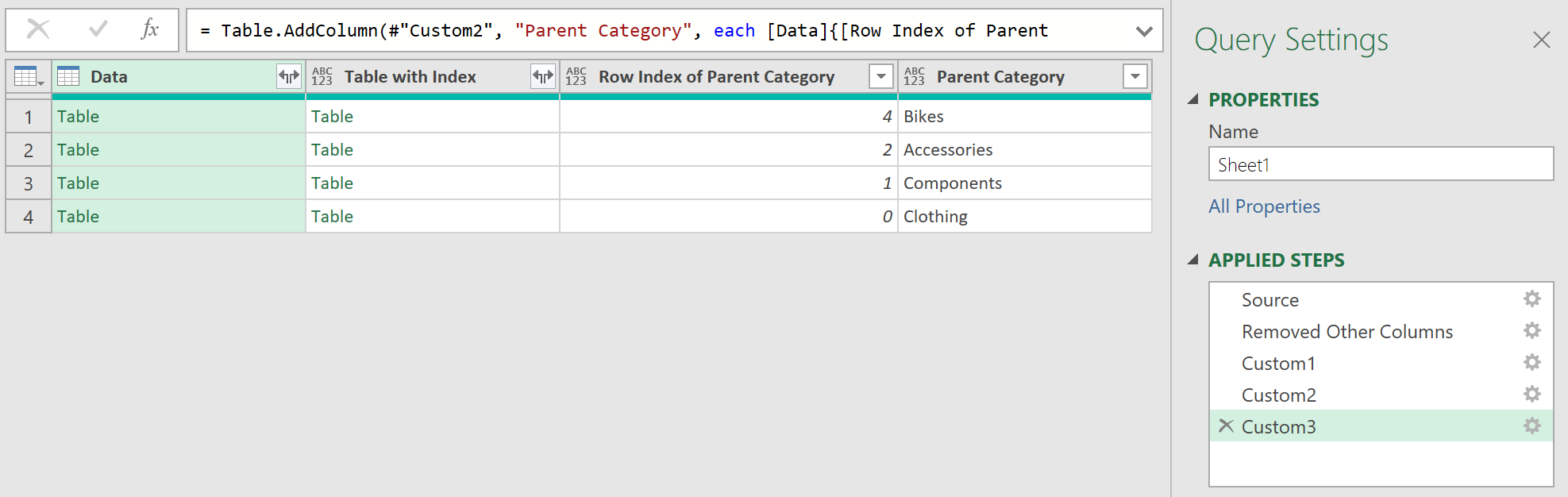
This returns the actual name of the Parent Category in a new column, called “Parent Category”.
6. Add row index of table data
- Next, add the following line of code:
= Table.AddColumn(#"Custom3", "Row Index of Name", each List.PositionOf([Data][Column1], "Name"))
The data should look like this:
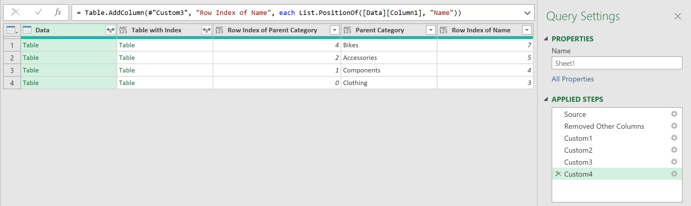
The line returns the row index of where the actual “Table Data” starts. Because of the inconsistent layouts across different files, the row index number will vary across the 4 separate sheets.
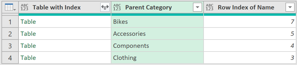
7. Remove irrelevant columns
- Next remove all columns so that you are only left with the following relevant columns:
8. Expand the data
- Next, expand the column called “Table with Index”, so that query returns the following data:
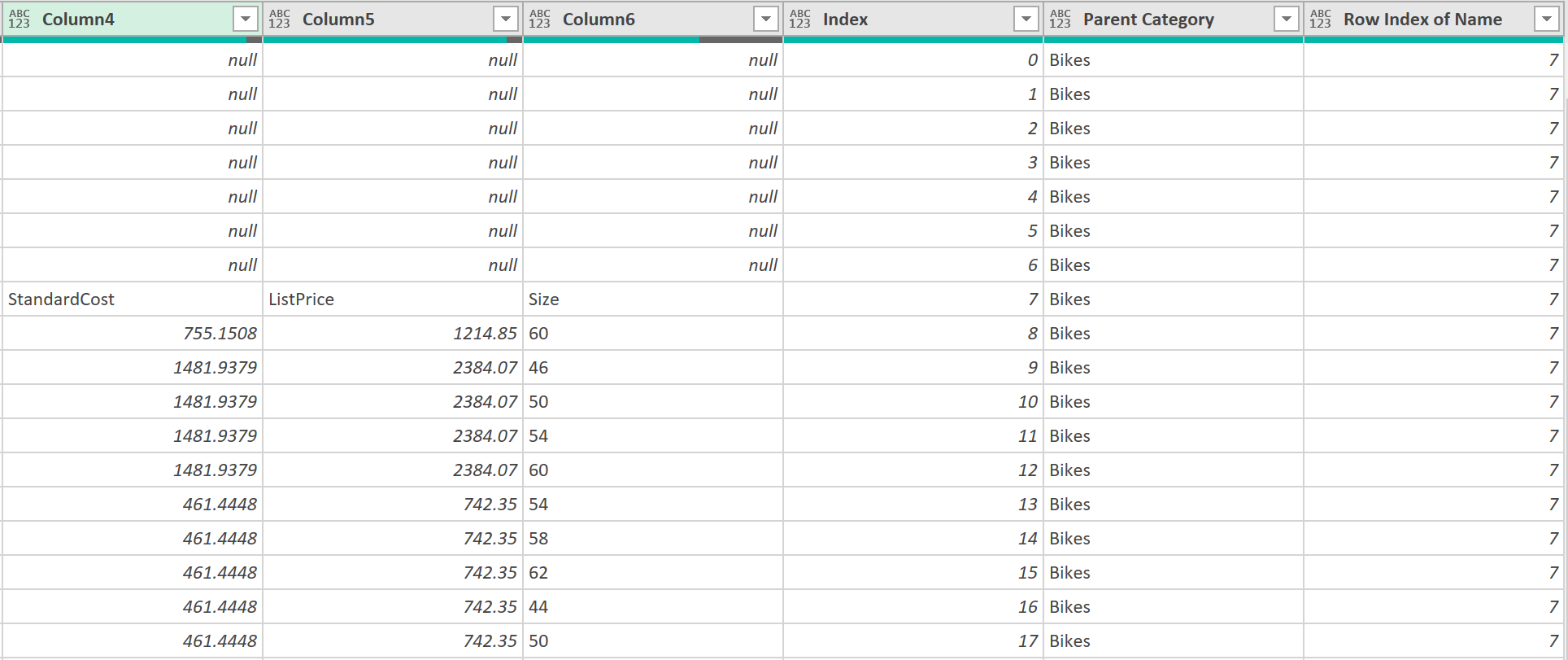
9. Filter out irrelevant rows
- Next, filter out the irrelevant rows.
- To do this, add the following conditional column, with the following parameters:
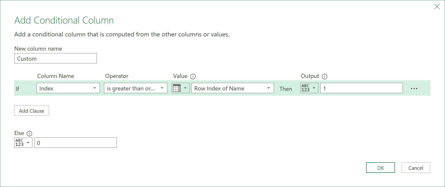
The conditional column will create an extra row, returning the number ‘1’ for all rows where the Index number is greater than the value in the column “Row Index of Name”. Refer to the picture below:
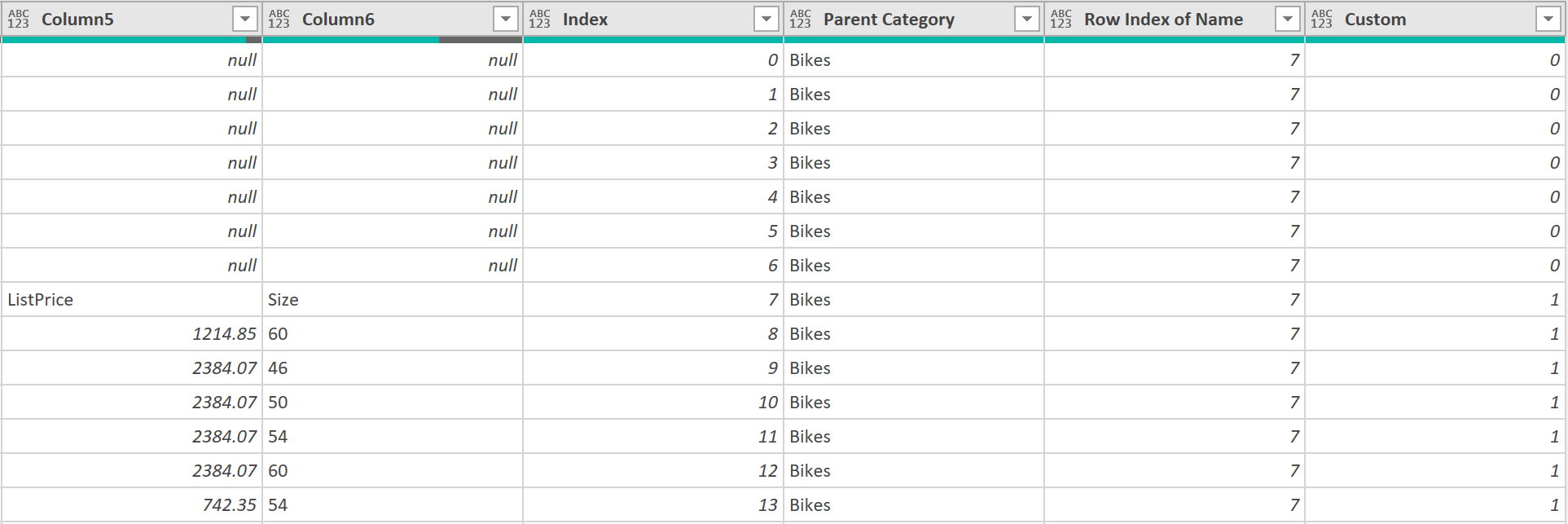
- Next, filter the “Custom” column to only include those rows with the number ‘1’.
- Then remove the columns called: “Index”, “Row Index of Name”, and “Custom”, so that the resulting query output looks as follows:
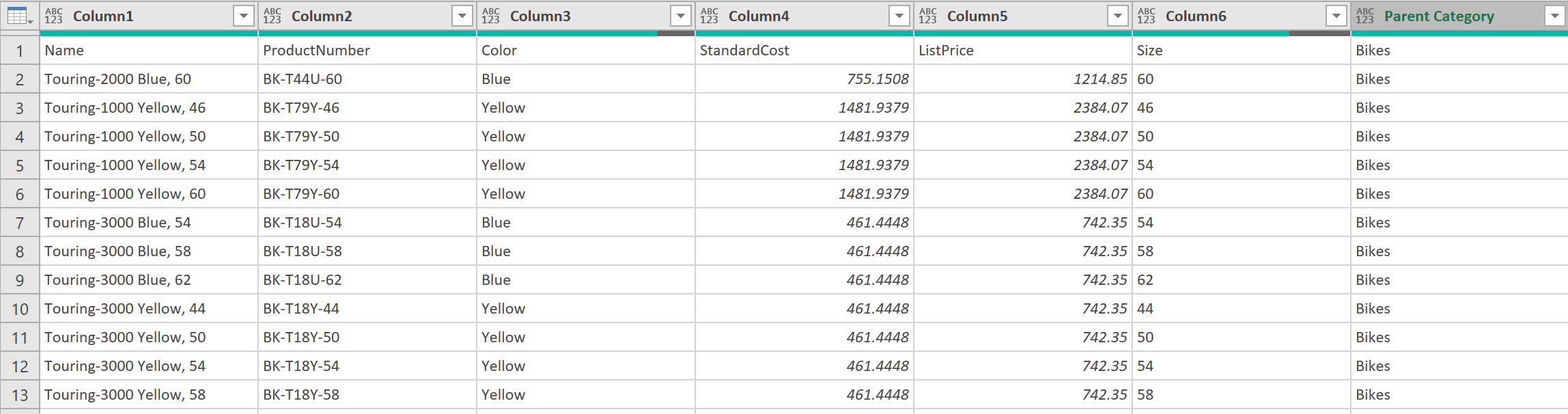
10. Tidy up data
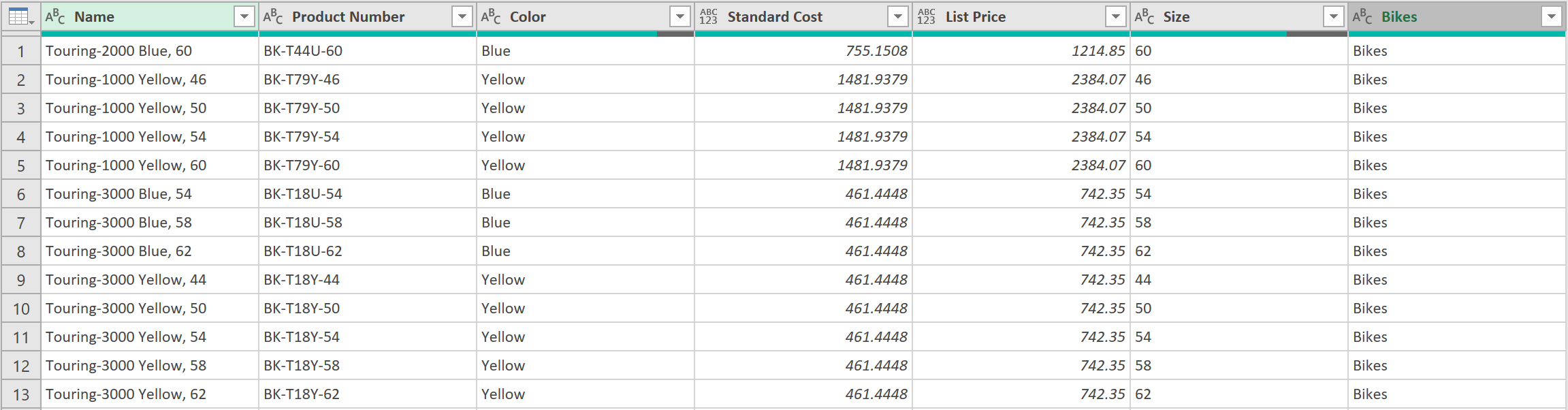
- After this, tidy up the data by: Promoting Headers, Setting Data Field Types, and Renaming the columns accordingly, to get to the output as shown below:
11. Filter out Header Rows
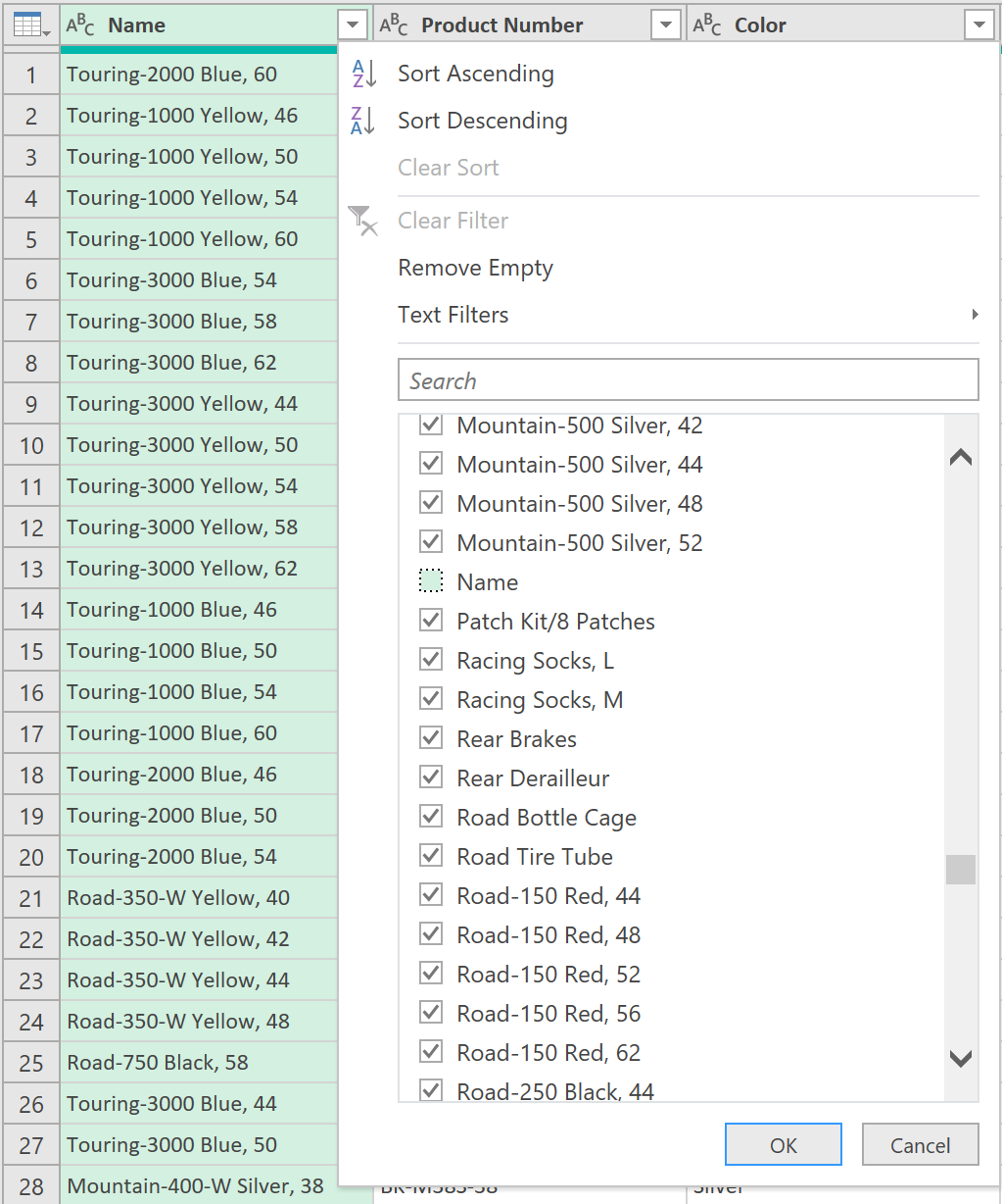
- Lastly, filter the column called “Name” to exclude any rows that are called “Name”, as shown below – and then you should be DONE!
12. Close & load
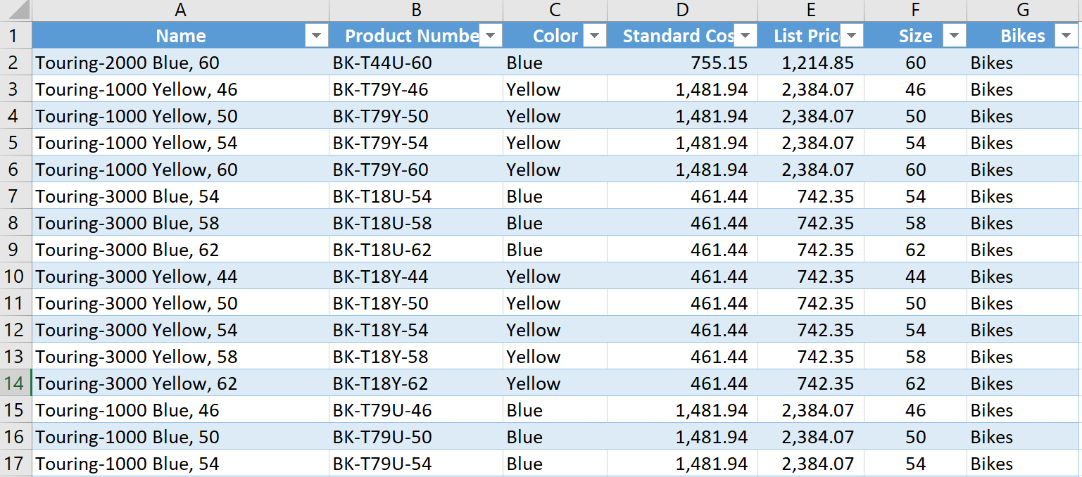
Finally, click Close & Load, so that the query loads the data – with the context - into the Excel Workbook – as shown below:
Final Comments
The technique uses cues to identify the proximity of the right context based on its proximity to “anchor” cells. Anchoring valuable data to fixed elements in your data, in this way, can vastly improve the robustness of your queries.
Here, the entire ETL process, when set up and tested thoroughly, (and provided well thought through and designed), should take no more than 5 minutes. Then you will probably want to leave another 3-4 minutes to quickly perform some “data checks” / “audit checks” back to the original data.
Feedback
Submit and view feedback