Tranforming Data into Tables

Overview

In the study of linguistics, scholars often distinguish between syntax, semantics, and pragmatics. While syntax focuses on the relationship between words, semantics deals with the meaning of sentences, pragmatics focuses on the way different contexts can influence the interpretation of a message - that is, the way you design your tables, significantly affects the way they are interpreted.

So just as where a different social context, or tone of voice, can affect the way a communicated message is interpreted, in data analytics, the design of tables can significantly affect the way it is analysed and interpreted.

In this article we show how any table, with a 2 x 2 level hierarchy, can be transformed into a form that the data in it can readily be analysed.

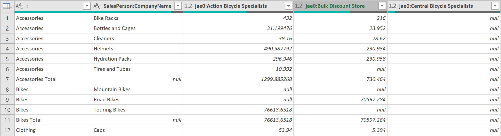
The figure below shows revenues, by sales person, by company name, for different product categories, and their sub-categories. Although the table does summarize information, it is not in a form that makes it easy to analyse.

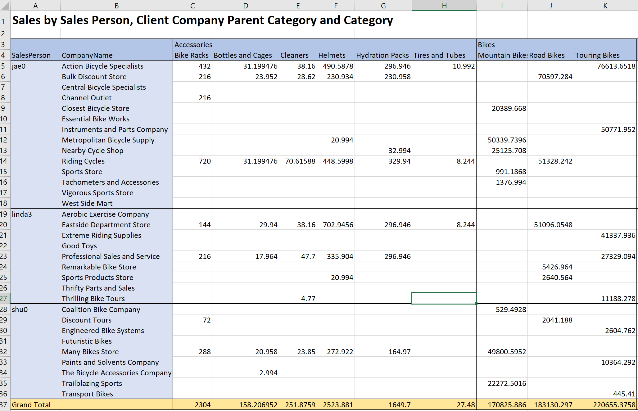
Instead we need to transform the table, by taking the following steps.

Steps

1. Load the data

• Open a new Excel File, and on the Data Tab, select ‘Get Data’, ‘From File’, ‘From Workbook’

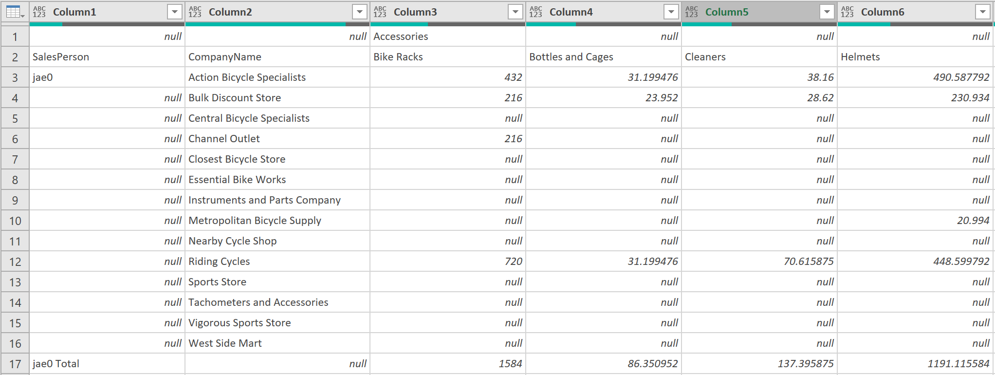
• Select the file called “Data with incorrect design.xlsx” – as shown below, and load it into the Query Editor so it looks like this:

• Click on the text that says ‘Table’ in the Data column, in the Revenues row, to load the revenue data, as shown below:

2. Remove Grand Total column

After loading the information, you should then remove the “Grand Total” column – which is the last column in the preview pane.

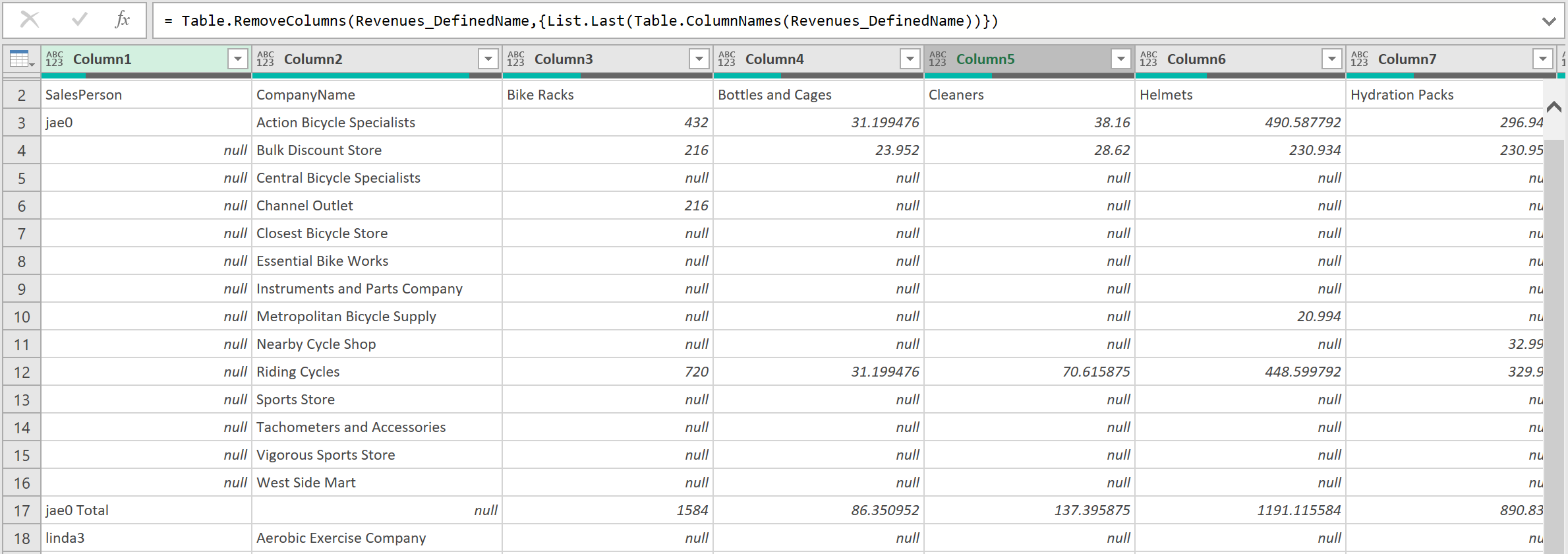
• Do not hard code this but do this dynamically by adding the following as an extra Applied Step – and as shown below.

   = Table.RemoveColumns(Revenues_DefinedName,{List.Last(Table.ColumnNames(Revenues_DefinedName))})

The data should look like this:

3. Remove Grant Total row

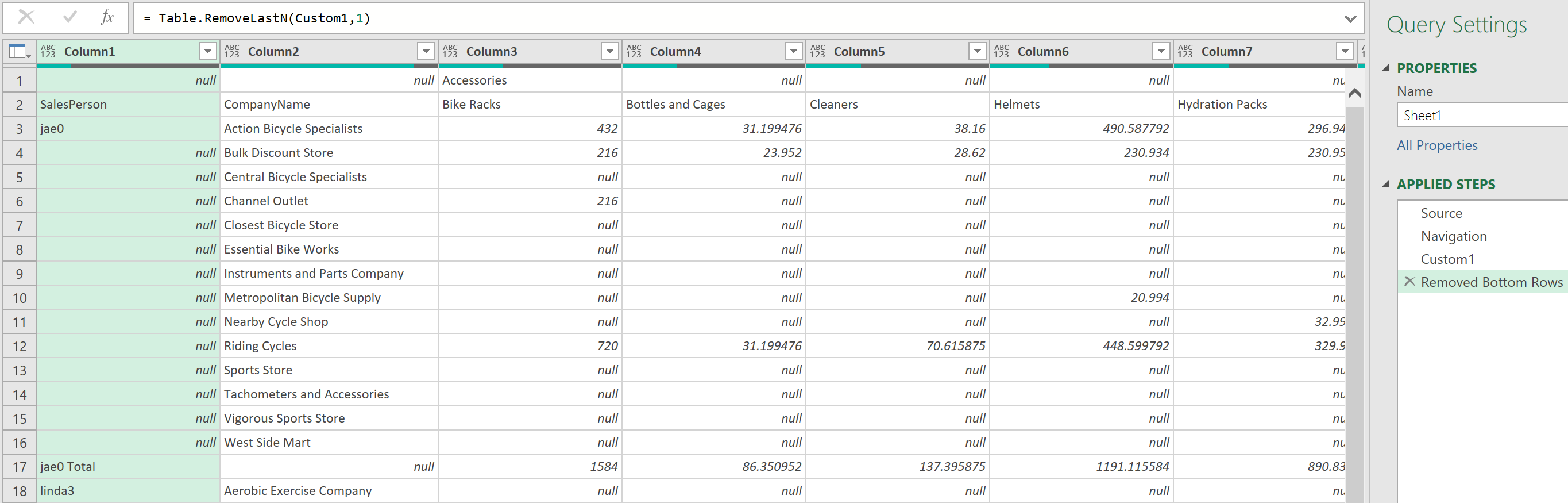
• After removing the “Grand Total” Column, remove the “Grand Total” row, - which is the bottom row, using the RemoveLastN function, as shown below:

4. Fill down the SalesPerson column

• Use the Fill Down function to fill down the blanks in the main anchor column, called SalesPerson - as shown below:

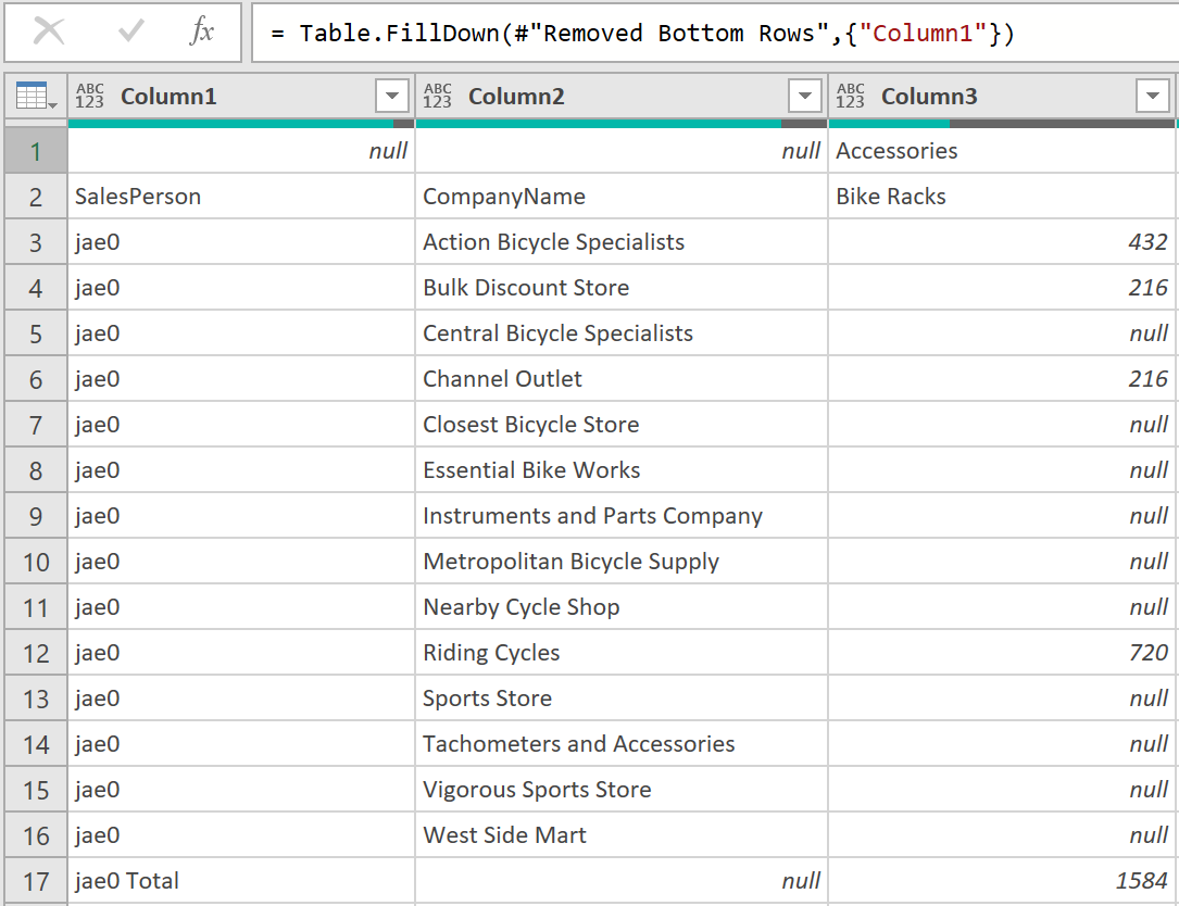
This should fill down the SalesPerson column and replace any null values with the correct values in each row.

5. Merge text columns

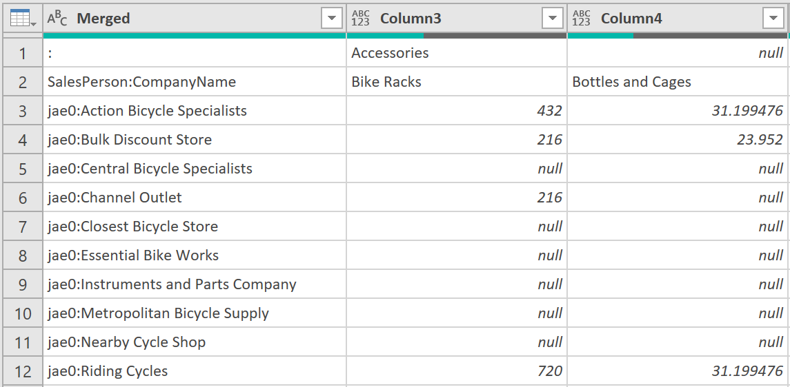
• After the Fill Down operation, use the Merged Columns function to merge Column1, and Column2.
• In the Merge Columns dialog box that opens, select Colon as the Separator, and then click OK to close the dialog box.

The data should look as follows:

6. Transpose the data table

• After Merging the two columns, on the Transform Tab, select Transpose, to transpose the whole table.

It should now look something like this:

7. Fill down the Category column

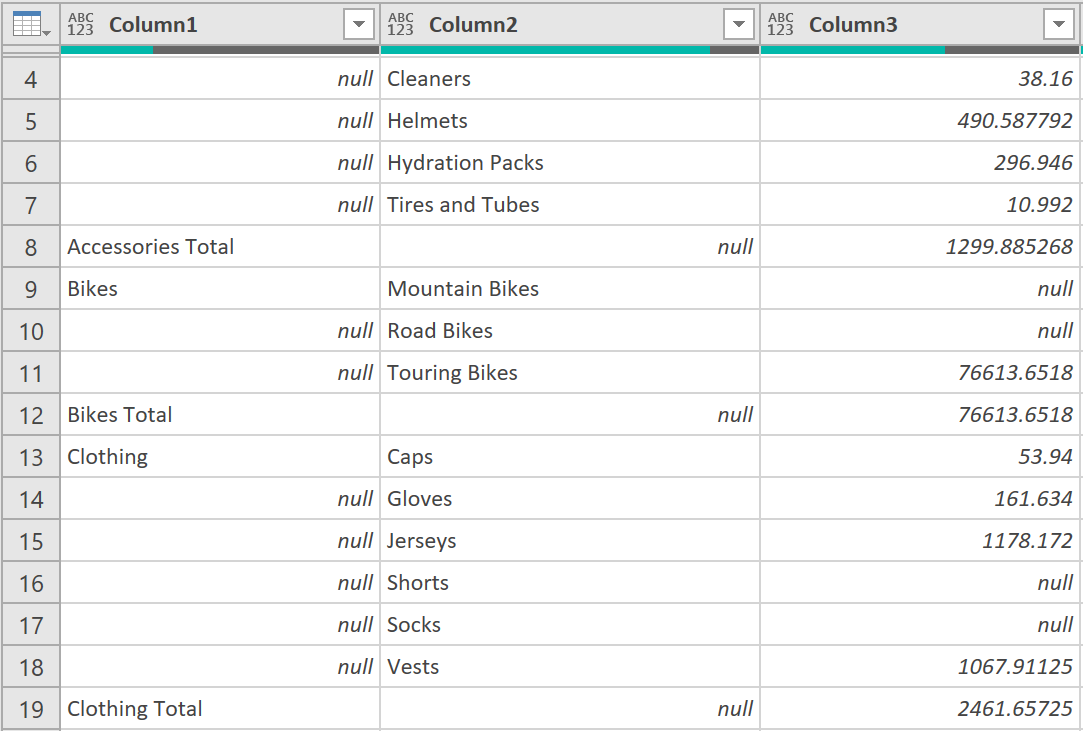
• Once Transposed, select the Fill Down function to fill out the gaps in the new anchor column (Product Category) – as shown below:

8. Promote Headers

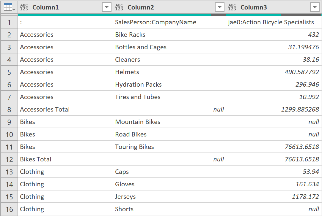
• After the second Fill Down operation, promote the top row as Headers – as shown below:

9. Unpivot the data table

• After this, select the first two columns above – those representing the product category, and supplier name.
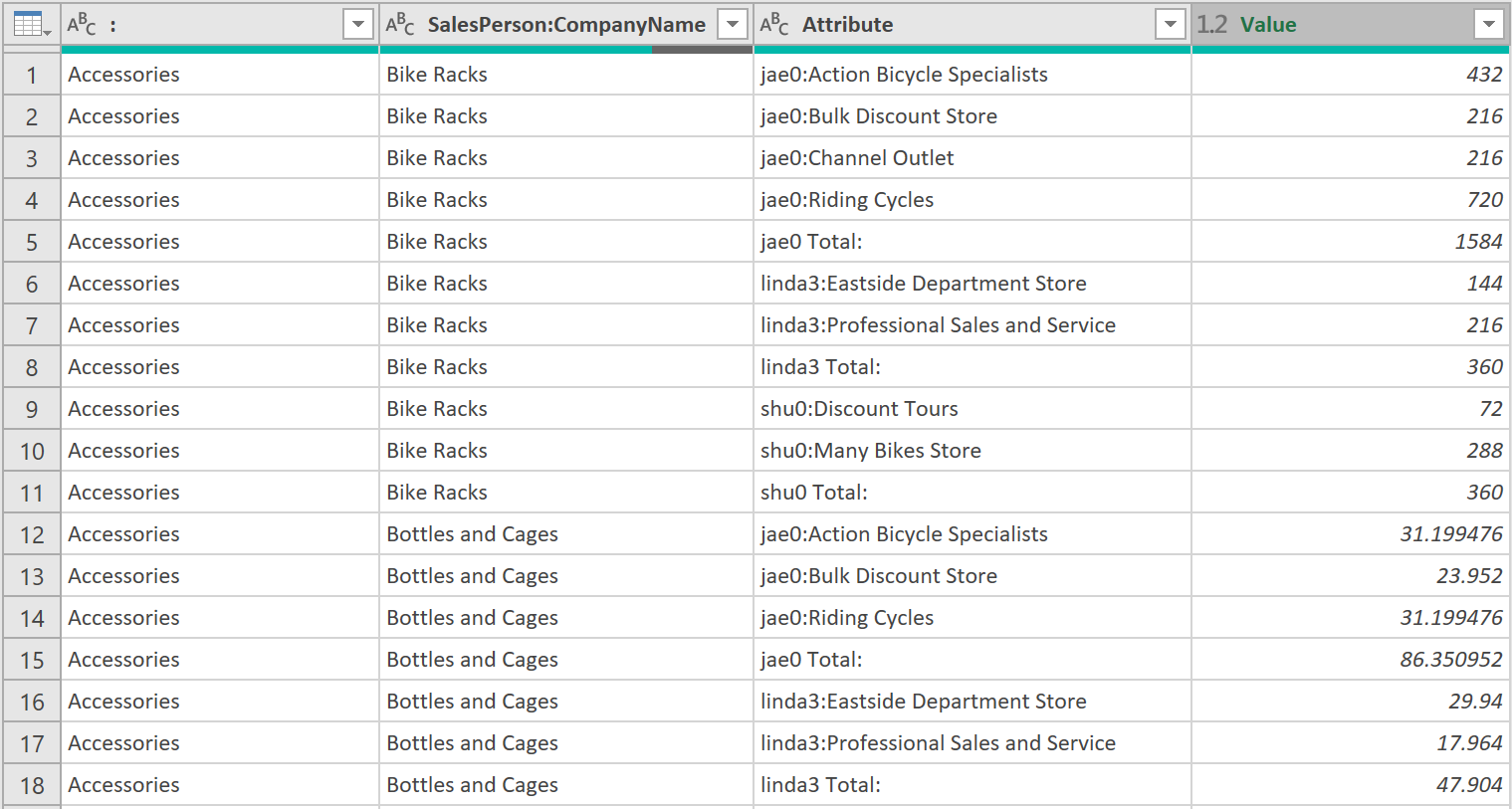
• Then on the Transform tab, click the Unpivot Columns drop-down menu, and then select Unpivot Other Columns

The data should now look like this:

10. Split columns

Now, fix the Attribute column – which, as it stands, consists of the merged SalesPerson, and CompanyName columns.

• To do this, select the Attribute column, and then on the Transform tab, select Split Column, By Delimiter.
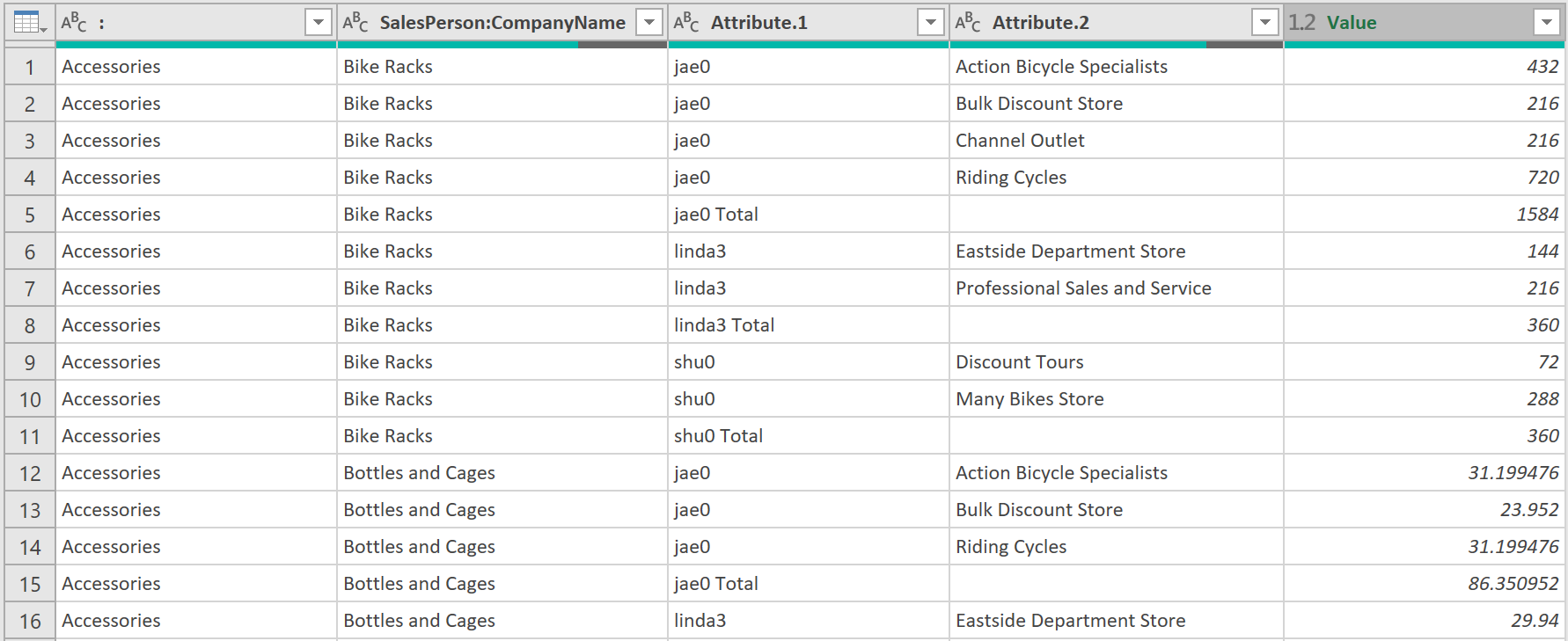
• In the Split Column By Delimiter dialog box that opens, set Select or Enter Delimiter to Colon, and then click Ok to close the dialog box.

The final result should look as follows:

11. Rename columns and filter out subtotals

• Rename the remaining columns to as follows:

1. First column: Parent Category
2. Second column: Category
3. Third column: Sales Person
4. Fourth column: Company
5. Fifth column: Revenue

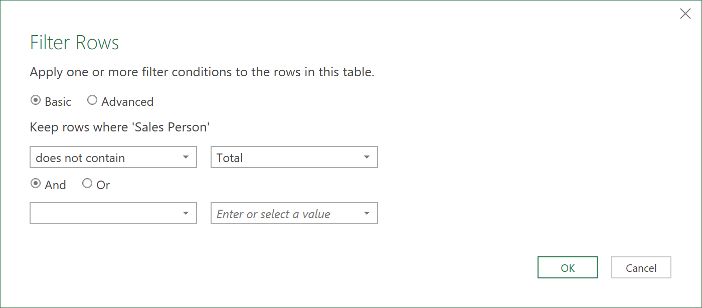
• Finally, filter out sub-totals in the Sales Person column, as follows:

12. Close & Load data

• Finally, on the Home tab, click Close and Load, to load the unpivoted data into the report – and Voila, you are done!

The data should look like this, in its final form:

Final Comments

Reiterating the linguistics analogy from earlier, with this ETL, we have moved from syntax, to semantics, to the realm of pragmatics. Essentially, here you should be aware of how different contexts can shape the perceived meaning of results.

To summarise what was carried out, the steps were to:

1. Remove any Grand Total columns, and rows,
2. Fill down the original anchor column,
3. Merge them into a single column,
4. Transpose the table,
5. Fill down the new anchor columns,
6. Select Use First Row as Headers,
7. Unpivot the data table,
8. Split the merged Attribute column,
9. Name the columns accordingly, and
10. Filter out the any subtotal rows.